Computer Vision Template matching and object recognition Marc
Computer Vision Template matching and object recognition Marc Pollefeys COMP 256 Some slides and illustrations from D. Forsyth, T. Tuytelaars, …
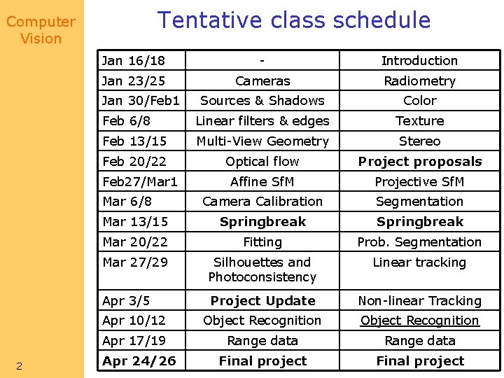
Tentative class schedule Computer Vision Jan 16/18 - Introduction Jan 23/25 Cameras Radiometry Sources & Shadows Color Feb 6/8 Linear filters & edges Texture Feb 13/15 Multi-View Geometry Stereo Feb 20/22 Optical flow Project proposals Affine Sf. M Projective Sf. M Camera Calibration Segmentation Mar 13/15 Springbreak Mar 20/22 Fitting Prob. Segmentation Mar 27/29 Silhouettes and Photoconsistency Linear tracking Apr 3/5 Project Update Non-linear Tracking Apr 10/12 Object Recognition Apr 17/19 Range data Final project Jan 30/Feb 1 Feb 27/Mar 1 Mar 6/8 2 Apr 24/26
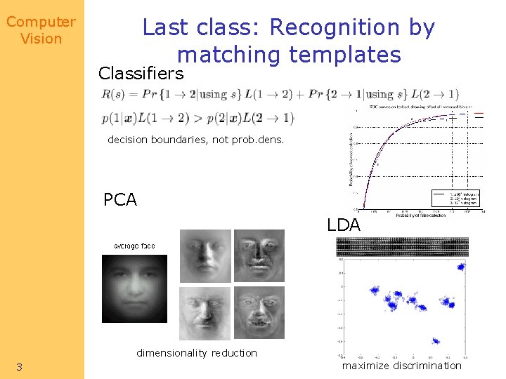
Computer Vision Last class: Recognition by matching templates Classifiers decision boundaries, not prob. dens. PCA LDA dimensionality reduction 3 maximize discrimination
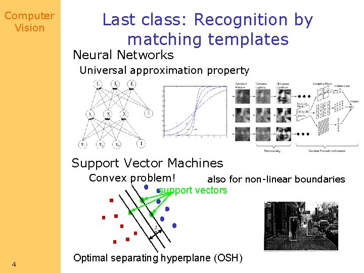
Computer Vision Last class: Recognition by matching templates Neural Networks Universal approximation property Support Vector Machines Convex problem! also for non-linear boundaries support vectors 4 Optimal separating hyperplane (OSH)
Computer Vision SVMs for 3 D object recognition (Pontil & Verri PAMI’ 98) - Consider images as vectors - Compute pairwise OSH using linear SVM - Support vectors are representative views of the considered object (relative to other) - Tournament like classification - Competing classes are grouped in pairs Not selected classes are discarded Until only one class is left Complexity linear in number of classes - No pose estimation 5
Computer Vision applications • Reliable, simple classifier, – use it wherever you need a classifier • Commonly used for face finding 6 • Pedestrian finding – many pedestrians look like lollipops (hands at sides, torso wider than legs) most of the time – classify image regions, searching over scales – But what are the features? – Compute wavelet coefficients for pedestrian windows, average over pedestrians. If the average is different from zero, probably strongly associated with pedestrian
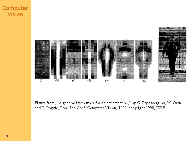
Computer Vision Figure from, “A general framework for object detection, ” by C. Papageorgiou, M. Oren and T. Poggio, Proc. Int. Conf. Computer Vision, 1998, copyright 1998, IEEE 7
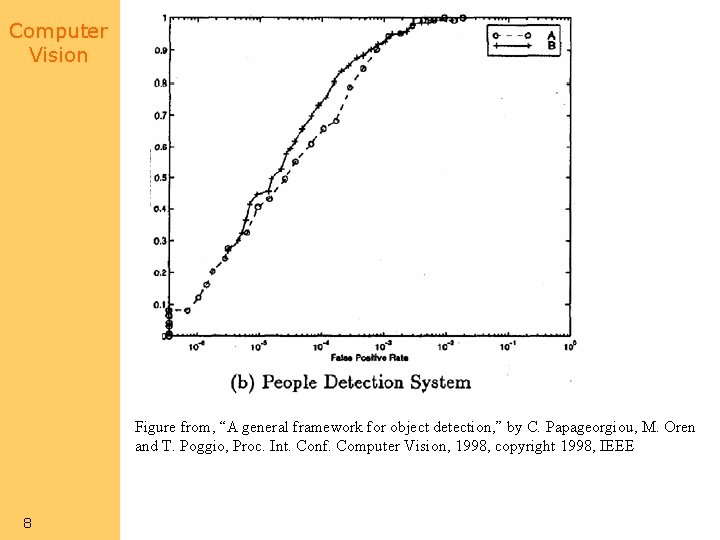
Computer Vision Figure from, “A general framework for object detection, ” by C. Papageorgiou, M. Oren and T. Poggio, Proc. Int. Conf. Computer Vision, 1998, copyright 1998, IEEE 8
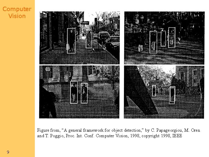
Computer Vision Figure from, “A general framework for object detection, ” by C. Papageorgiou, M. Oren and T. Poggio, Proc. Int. Conf. Computer Vision, 1998, copyright 1998, IEEE 9

Computer Vision Latest results on Pedestrian Detection: Viola, Jones and Snow’s paper (ICCV’ 03: Marr prize) • Combine static and dynamic features cascade for efficiency (4 frames/s) 5 best out of 55 k (Ada. Boost) 10 some positive examples used for training 5 best static out of 28 k (Ada. Boost)
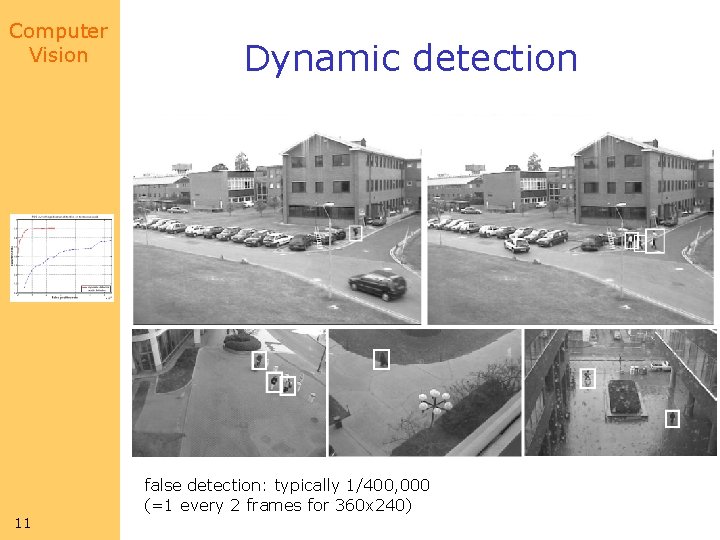
Computer Vision Dynamic detection false detection: typically 1/400, 000 (=1 every 2 frames for 360 x 240) 11
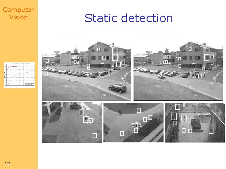
Computer Vision 12 Static detection
Computer Vision Matching by relations • Idea: – find bits, then say object is present if bits are ok • Advantage: – objects with complex configuration spaces don’t make good templates • • • 13 internal degrees of freedom aspect changes (possibly) shading variations in texture etc.
Computer Vision Simplest • Define a set of local feature templates – could find these with filters, etc. – corner detector+filters • Think of objects as patterns • Each template votes for all patterns that contain it • Pattern with the most votes wins 14
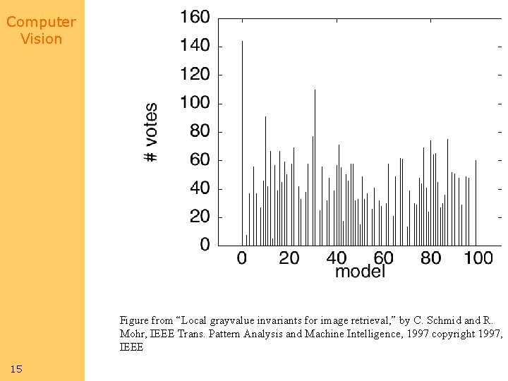
Computer Vision Figure from “Local grayvalue invariants for image retrieval, ” by C. Schmid and R. Mohr, IEEE Trans. Pattern Analysis and Machine Intelligence, 1997 copyright 1997, IEEE 15
Computer Vision Probabilistic interpretation • Write • Assume • Likelihood of image given pattern 16
Computer Vision Possible alternative strategies • Notice: – different patterns may yield different templates with different probabilities – different templates may be found in noise with different probabilities 17
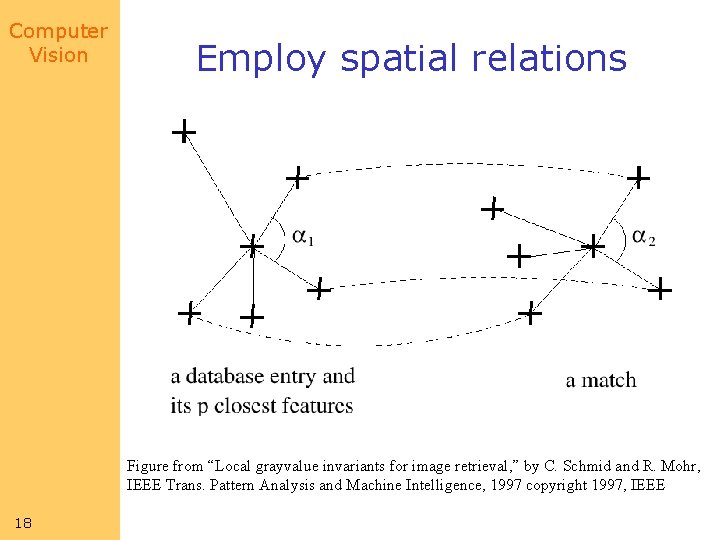
Computer Vision Employ spatial relations Figure from “Local grayvalue invariants for image retrieval, ” by C. Schmid and R. Mohr, IEEE Trans. Pattern Analysis and Machine Intelligence, 1997 copyright 1997, IEEE 18
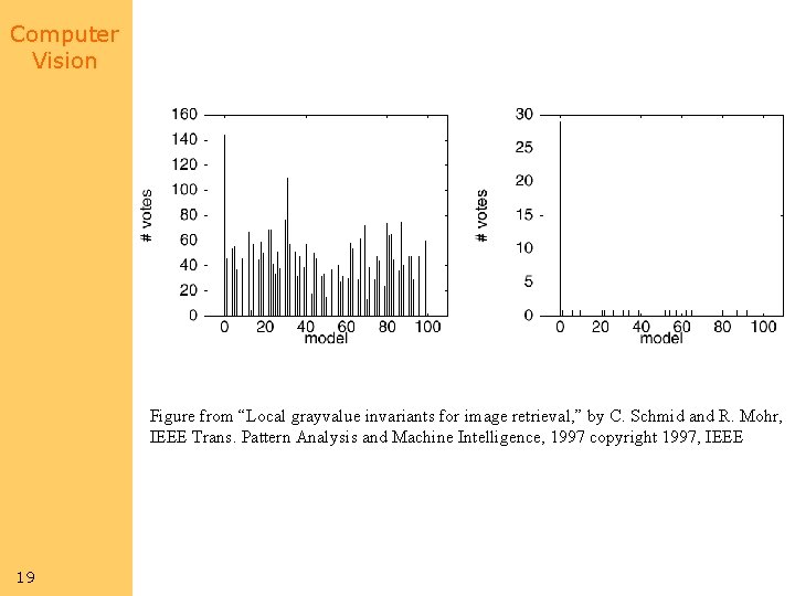
Computer Vision Figure from “Local grayvalue invariants for image retrieval, ” by C. Schmid and R. Mohr, IEEE Trans. Pattern Analysis and Machine Intelligence, 1997 copyright 1997, IEEE 19
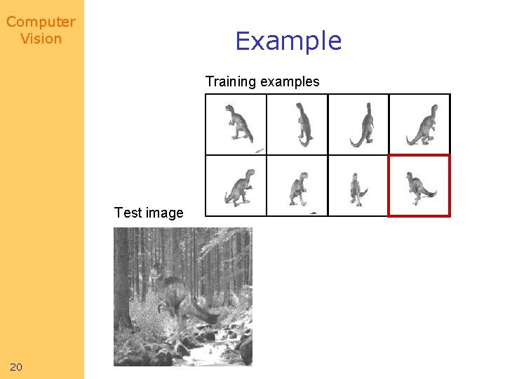
Computer Vision Example Training examples Test image 20
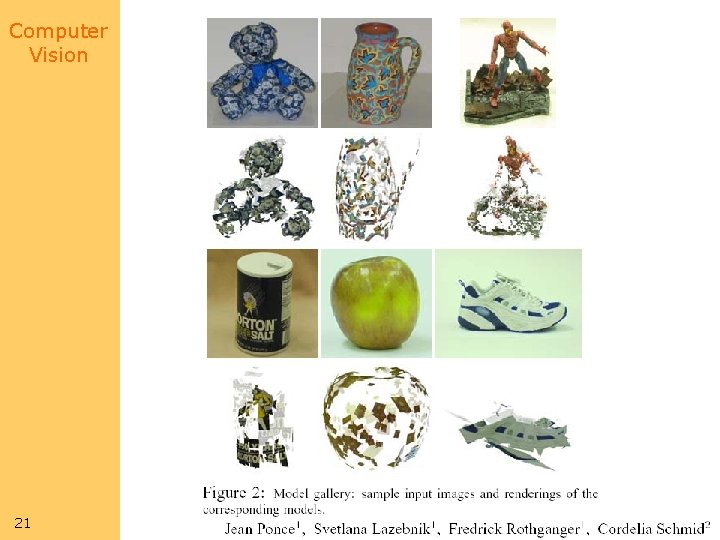
Computer Vision 21
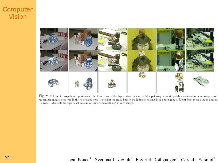
Computer Vision 22
Computer Vision Finding faces using relations • Strategy: – Face is eyes, nose, mouth, etc. with appropriate relations between them – build a specialised detector for each of these (template matching) and look for groups with the right internal structure – Once we’ve found enough of a face, there is little uncertainty about where the other bits could be 23
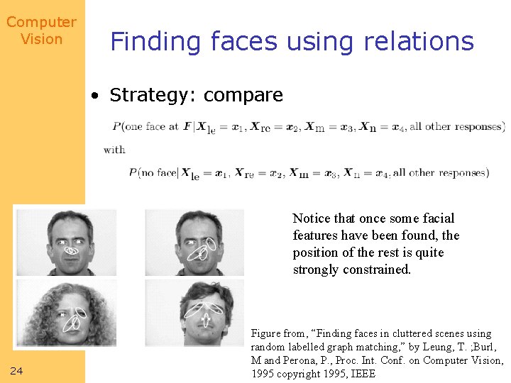
Computer Vision Finding faces using relations • Strategy: compare Notice that once some facial features have been found, the position of the rest is quite strongly constrained. 24 Figure from, “Finding faces in cluttered scenes using random labelled graph matching, ” by Leung, T. ; Burl, M and Perona, P. , Proc. Int. Conf. on Computer Vision, 1995 copyright 1995, IEEE
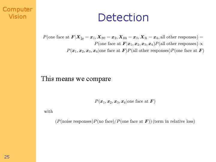
Computer Vision Detection This means we compare 25
Computer Vision Issues • Plugging in values for position of nose, eyes, etc. – search for next one given what we’ve found • when to stop searching – when nothing that is added to the group could change the decision – i. e. it’s not a face, whatever features are added or – it’s a face, and anything you can’t find is occluded • what to do next – look for another eye? or a nose? – probably look for the easiest to find • What if there’s no nose response – marginalize 26
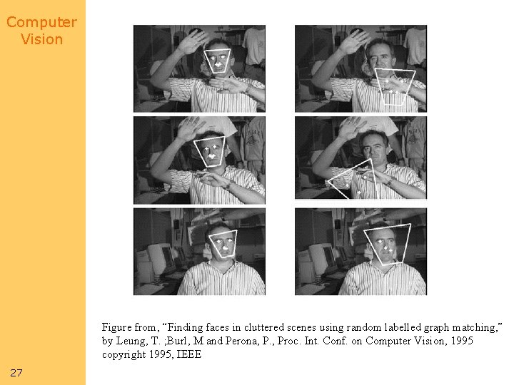
Computer Vision Figure from, “Finding faces in cluttered scenes using random labelled graph matching, ” by Leung, T. ; Burl, M and Perona, P. , Proc. Int. Conf. on Computer Vision, 1995 copyright 1995, IEEE 27
Computer Vision Pruning • Prune using a classifier – crude criterion: if this small assembly doesn’t work, there is no need to build on it. 28 • Example: finding people without clothes on – find skin – find extended skin regions – construct groups that pass local classifiers (i. e. lower arm, upper arm) – give these to broader scale classifiers (e. g. girdle)
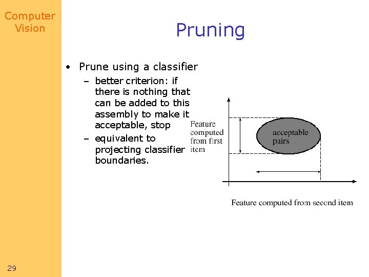
Computer Vision Pruning • Prune using a classifier – better criterion: if there is nothing that can be added to this assembly to make it acceptable, stop – equivalent to projecting classifier boundaries. 29
Computer Vision 30 Horses
Computer Vision Hidden Markov Models • Elements of sign language understanding – the speaker makes a sequence of signs – Some signs are more common than others – the next sign depends (roughly, and probabilistically) only on the current sign – there are measurements, which may be inaccurate; different signs tend to generate different probability densities on measurement values • Many problems share these properties – tracking is like this, for example 31
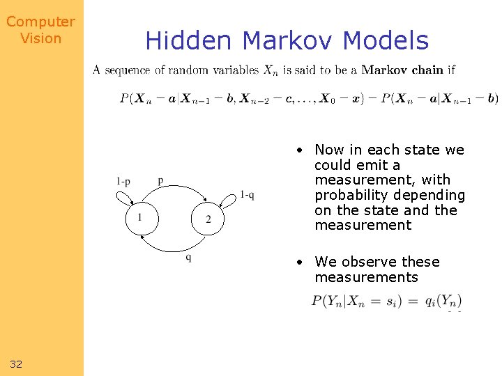
Computer Vision Hidden Markov Models • Now in each state we could emit a measurement, with probability depending on the state and the measurement • We observe these measurements 32
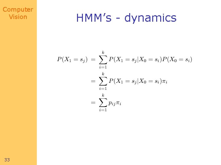
Computer Vision 33 HMM’s - dynamics
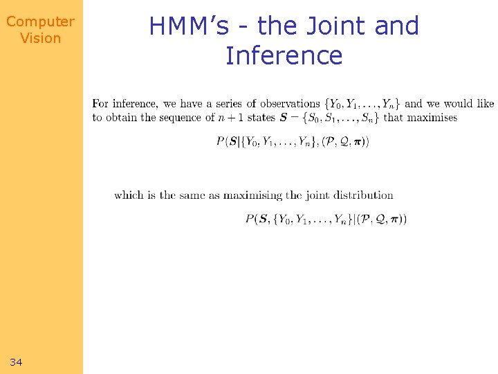
Computer Vision 34 HMM’s - the Joint and Inference
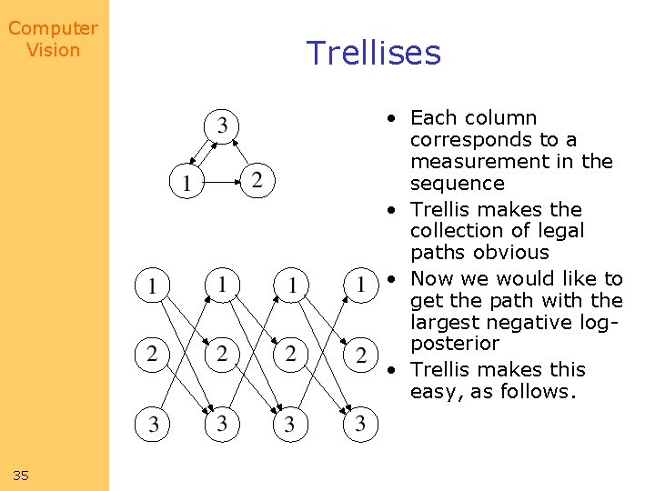
Computer Vision Trellises • Each column corresponds to a measurement in the sequence • Trellis makes the collection of legal paths obvious • Now we would like to get the path with the largest negative logposterior • Trellis makes this easy, as follows. 35
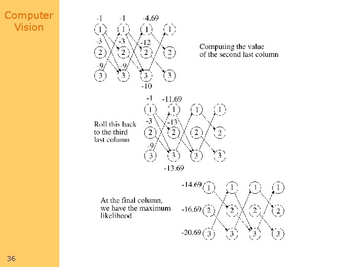
Computer Vision 36
Computer Vision Fitting an HMM • I have: – sequence of measurements – collection of states – topology • I want – state transition probabilities – measurement emission probabilities • Straightforward application of EM – discrete vars give state for each measurement – M step is just averaging, etc. 37
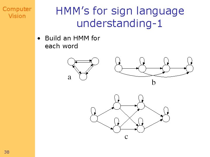
Computer Vision HMM’s for sign language understanding-1 • Build an HMM for each word 38
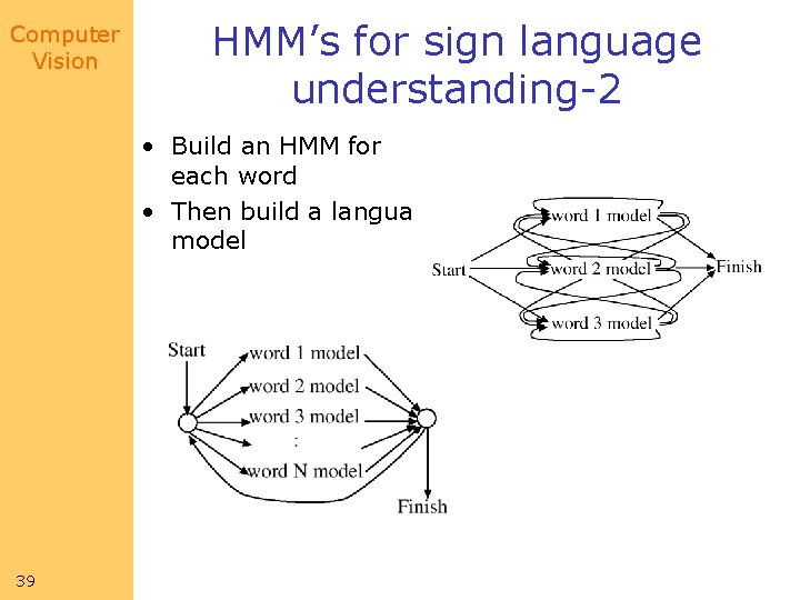
Computer Vision HMM’s for sign language understanding-2 • Build an HMM for each word • Then build a language model 39
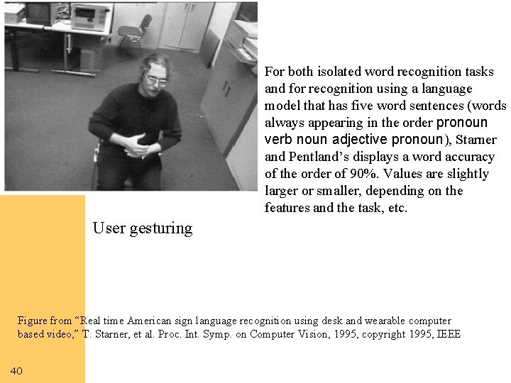
Computer Vision For both isolated word recognition tasks and for recognition using a language model that has five word sentences (words always appearing in the order pronoun verb noun adjective pronoun), Starner and Pentland’s displays a word accuracy of the order of 90%. Values are slightly larger or smaller, depending on the features and the task, etc. User gesturing Figure from “Real time American sign language recognition using desk and wearable computer based video, ” T. Starner, et al. Proc. Int. Symp. on Computer Vision, 1995, copyright 1995, IEEE 40
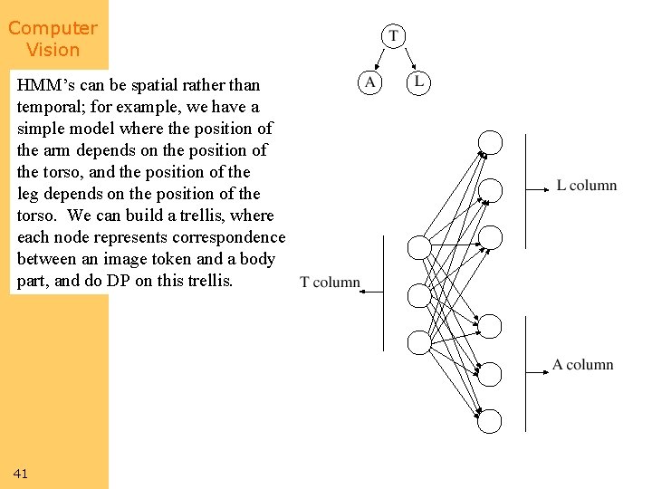
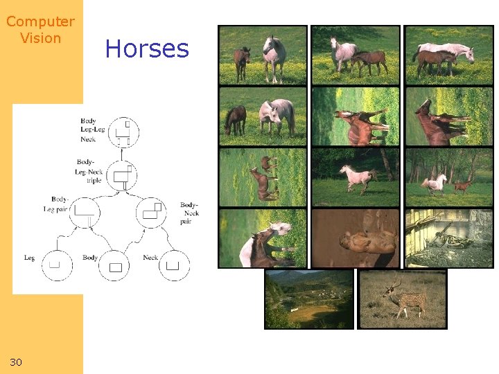
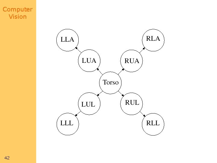
Computer Vision HMM’s can be spatial rather than temporal; for example, we have a simple model where the position of the arm depends on the position of the torso, and the position of the leg depends on the position of the torso. We can build a trellis, where each node represents correspondence between an image token and a body part, and do DP on this trellis. 41
Computer Vision 42
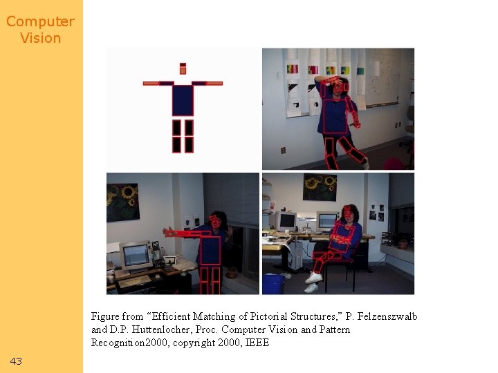
Computer Vision Figure from “Efficient Matching of Pictorial Structures, ” P. Felzenszwalb and D. P. Huttenlocher, Proc. Computer Vision and Pattern Recognition 2000, copyright 2000, IEEE 43
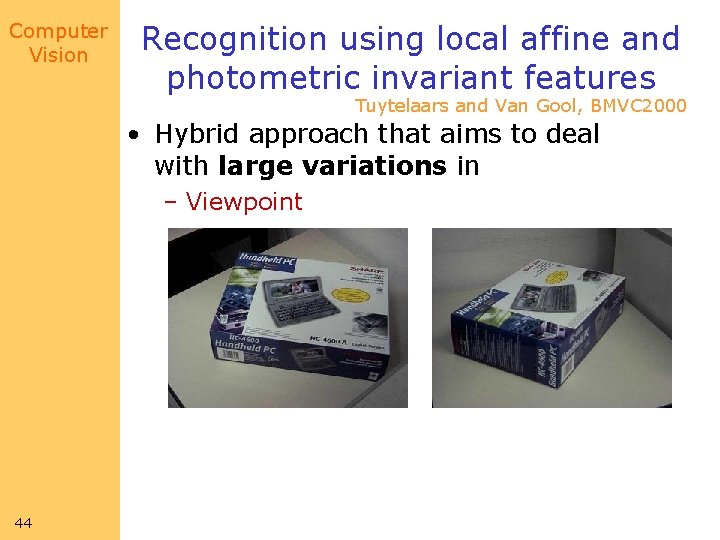
Computer Vision Recognition using local affine and photometric invariant features Tuytelaars and Van Gool, BMVC 2000 • Hybrid approach that aims to deal with large variations in – Viewpoint 44
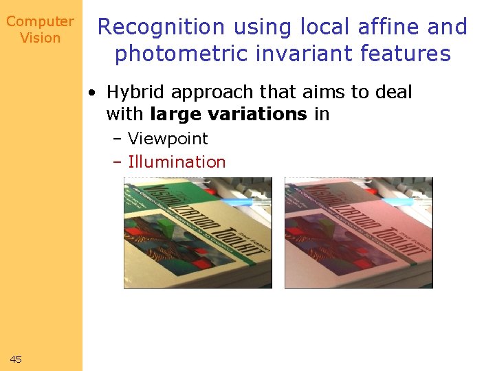
Computer Vision Recognition using local affine and photometric invariant features • Hybrid approach that aims to deal with large variations in – Viewpoint – Illumination 45
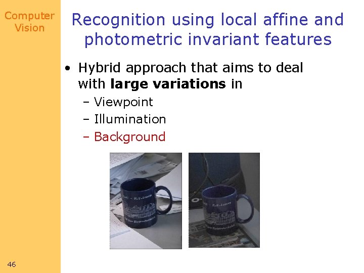
Computer Vision Recognition using local affine and photometric invariant features • Hybrid approach that aims to deal with large variations in – Viewpoint – Illumination – Background 46
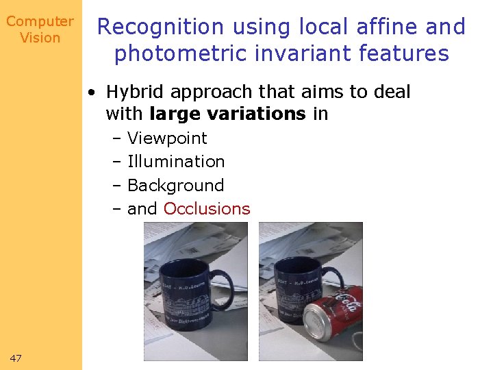
Computer Vision Recognition using local affine and photometric invariant features • Hybrid approach that aims to deal with large variations in – Viewpoint – Illumination – Background – and Occlusions 47
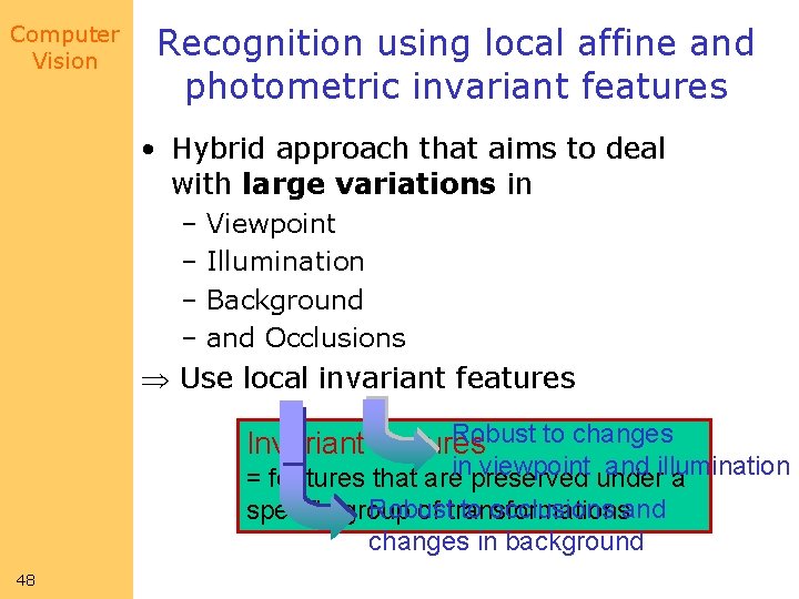
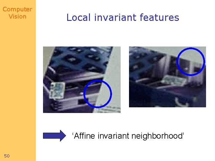
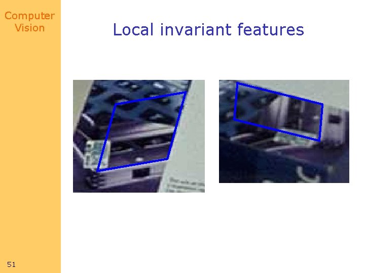
Computer Vision Recognition using local affine and photometric invariant features • Hybrid approach that aims to deal with large variations in – Viewpoint – Illumination – Background – and Occlusions Use local invariant features Robust to changes Invariant features viewpoint under and illumination = features that areinpreserved a Robust to occlusions and specific group of transformations changes in background 48
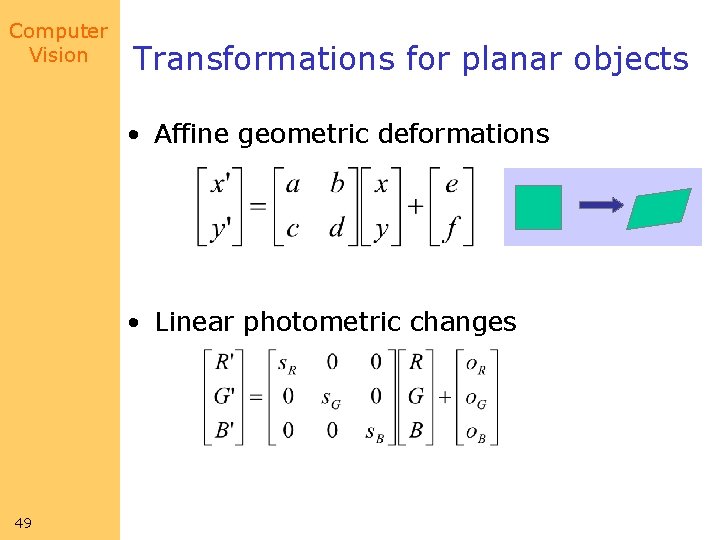
Computer Vision Transformations for planar objects • Affine geometric deformations • Linear photometric changes 49
Computer Vision Local invariant features ‘Affine invariant neighborhood’ 50
Computer Vision 51 Local invariant features
Computer Vision Local invariant features • Geometry-based region extraction – Curved edges – Straight edges • Intensity-based region extraction 52
Computer Vision 53 Geometry-based method (curved edges)
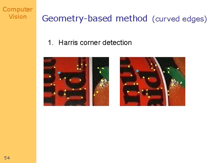
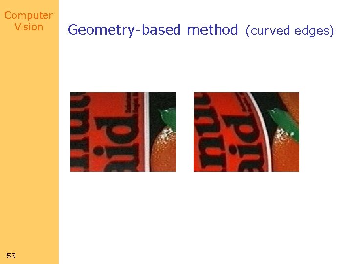
Computer Vision Geometry-based method (curved edges) 1. Harris corner detection 54
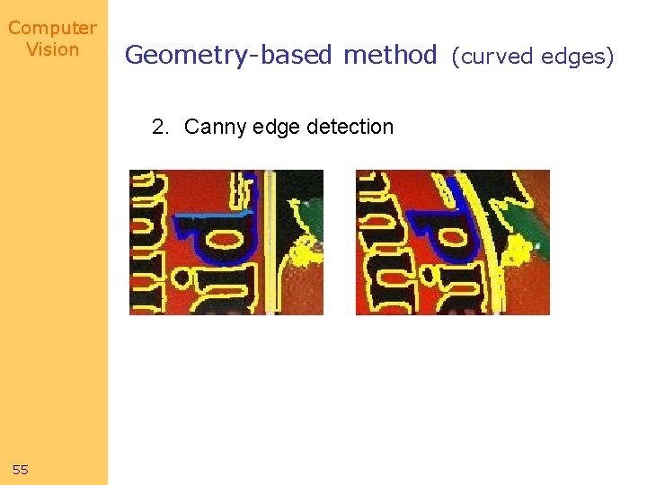
Computer Vision Geometry-based method (curved edges) 2. Canny edge detection 55
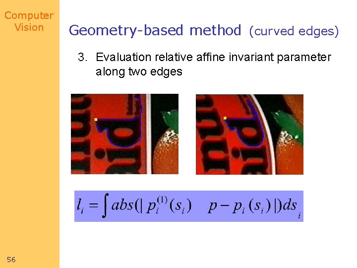
Computer Vision Geometry-based method (curved edges) 3. Evaluation relative affine invariant parameter along two edges 56
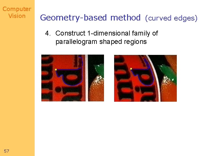
Computer Vision Geometry-based method (curved edges) 4. Construct 1 -dimensional family of parallelogram shaped regions 57
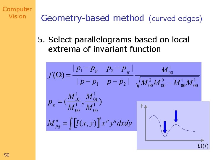
Computer Vision Geometry-based method (curved edges) 5. Select parallelograms based on local extrema of invariant function f 58
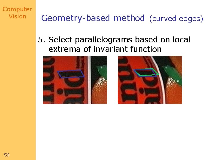
Computer Vision Geometry-based method (curved edges) 5. Select parallelograms based on local extrema of invariant function 59
Computer Vision Geometry-based method (straight edges) • Relative affine invariant parameters are identically zero! 60
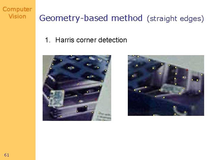
Computer Vision Geometry-based method (straight edges) 1. Harris corner detection 61
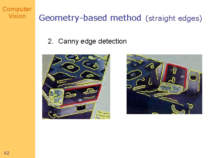
Computer Vision Geometry-based method (straight edges) 2. Canny edge detection 62
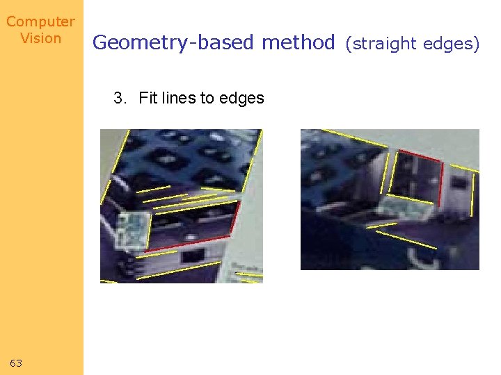
Computer Vision Geometry-based method (straight edges) 3. Fit lines to edges 63
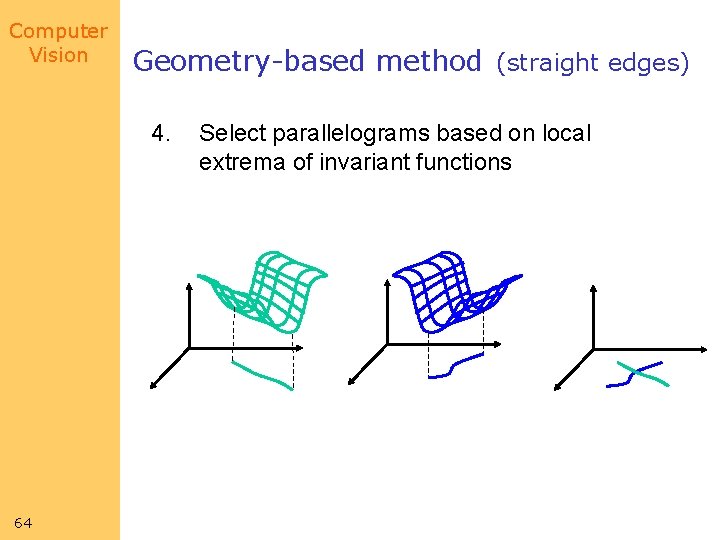
Computer Vision Geometry-based method (straight edges) 4. 64 Select parallelograms based on local extrema of invariant functions
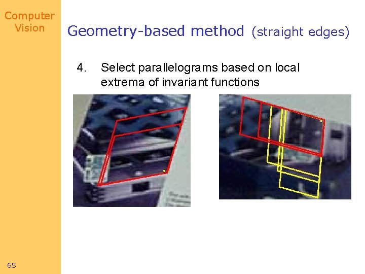
Computer Vision Geometry-based method (straight edges) 4. 65 Select parallelograms based on local extrema of invariant functions
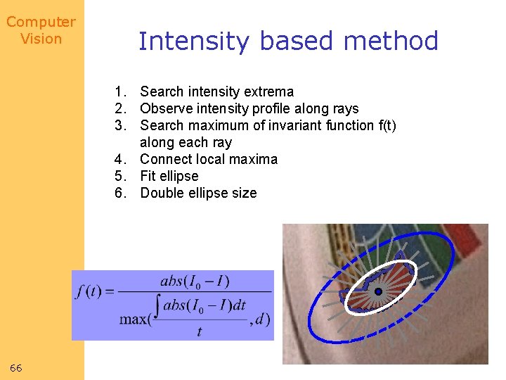
Computer Vision Intensity based method 1. Search intensity extrema 2. Observe intensity profile along rays 3. Search maximum of invariant function f(t) along each ray 4. Connect local maxima 5. Fit ellipse 6. Double ellipse size 66
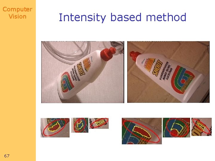
Computer Vision 67 Intensity based method
Computer Vision Comparison Intensity-based method • More robust Geometry-based method • Less computations • More environments 68
Computer Vision Robustness • “Correct” detection of single environment cannot be guaranteed – – – Non-planar region Noise, quantization errors Non-linear photometric distortion Perspective-distortion … All regions of an object / image should be considered simultaneously 69
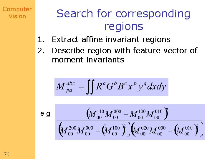
Computer Vision Search for corresponding regions 1. Extract affine invariant regions 2. Describe region with feature vector of moment invariants e. g. 70
Computer Vision Search for corresponding regions 1. Extract affine invariant regions 2. Describe region with feature vector of moment invariants 3. Search for corresponding regions based on Mahalanobis distance 4. Check cross-correlation (after normalization) 5. Check consistency of correspondences 71
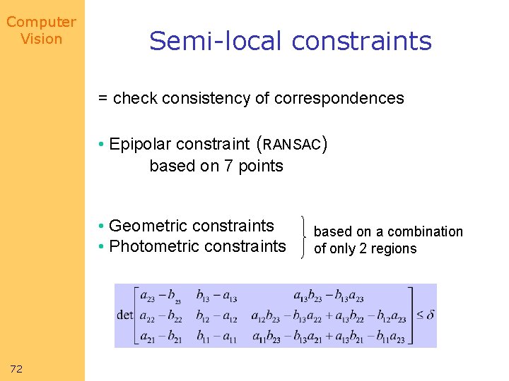
Computer Vision Semi-local constraints = check consistency of correspondences • Epipolar constraint (RANSAC) based on 7 points • Geometric constraints • Photometric constraints 72 based on a combination of only 2 regions
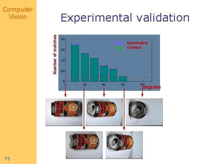
Computer Vision Number of matches Experimental validation symmetric correct degrees 73
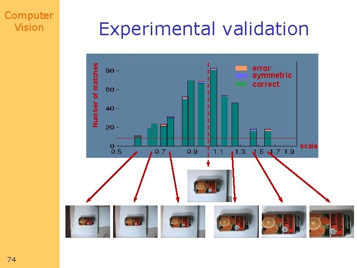
Experimental validation Number of matches Computer Vision error symmetric correct scale 74
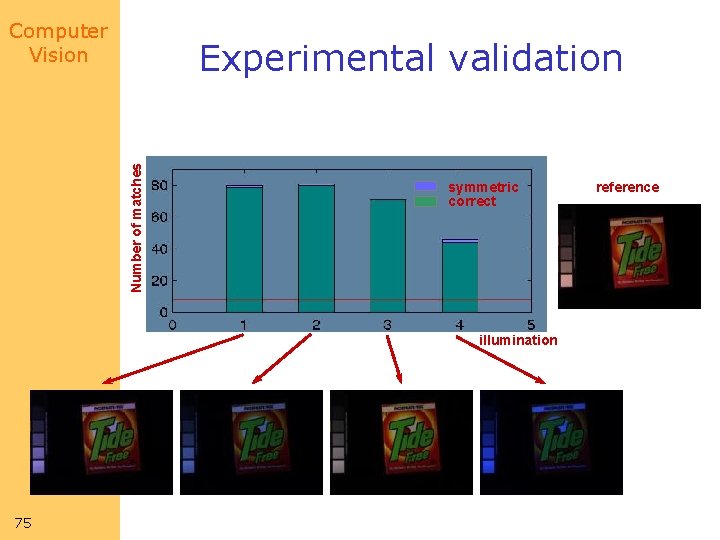
Computer Vision Number of matches Experimental validation symmetric correct illumination 75 reference
Computer Vision Object recognition and localization • ‘Appearance’-based approach = objects are modeled by a set of reference images Voting principle based on number of similar regions More invariance = requires less reference images 76
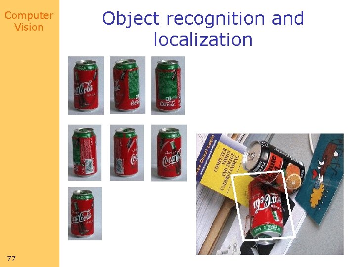
Computer Vision 77 Object recognition and localization
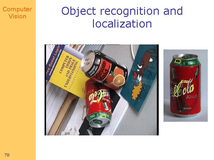
Computer Vision 78 Object recognition and localization
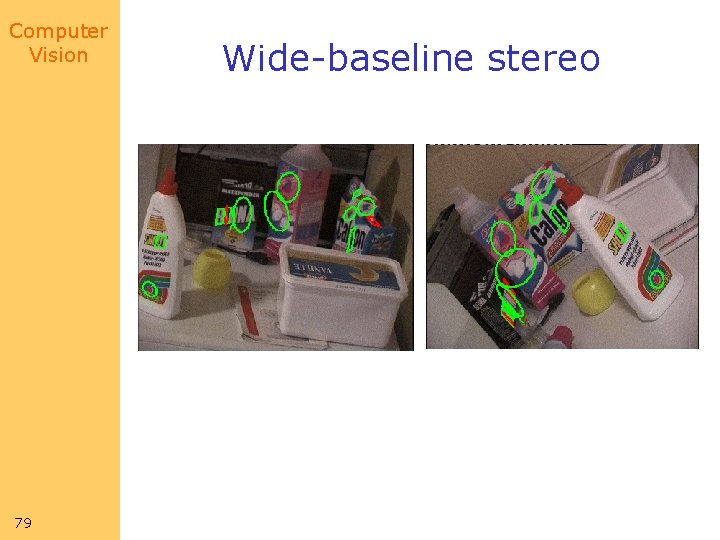
Computer Vision 79 Wide-baseline stereo
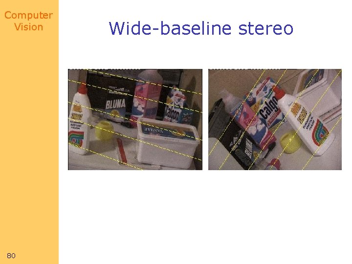
Computer Vision 80 Wide-baseline stereo
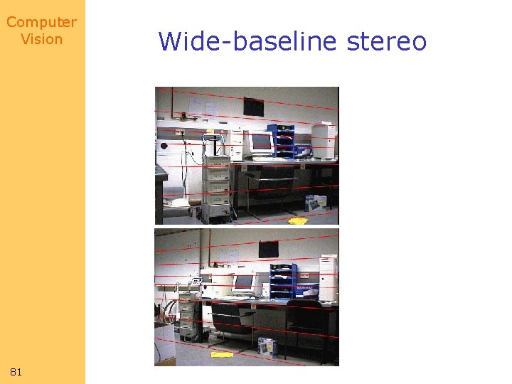
Computer Vision 81 Wide-baseline stereo
Computer Vision Content-based image retrieval from database • = Searching of ‘similar’ images in a databased on image content • Local features • Similarity = images contain the same object or the same scene • Voting principle – Based on the number of similar regions 82
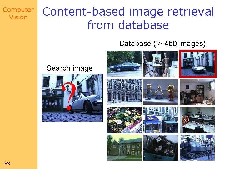
Computer Vision Content-based image retrieval from database Database ( > 450 images) Search image 83
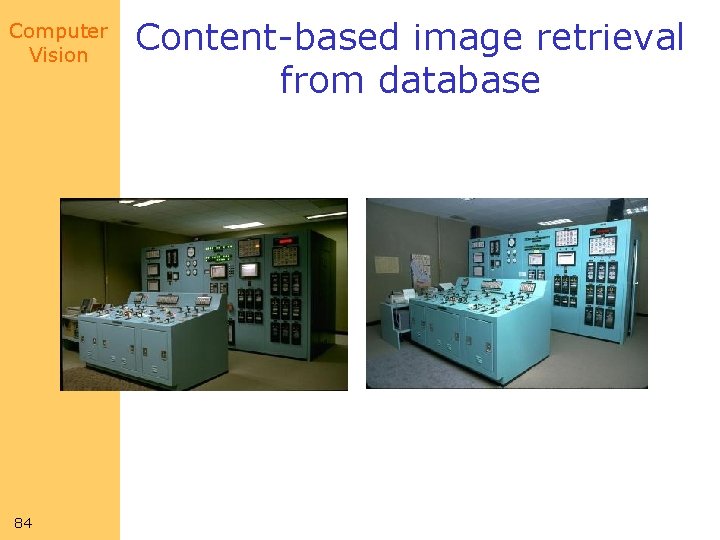
Computer Vision 84 Content-based image retrieval from database
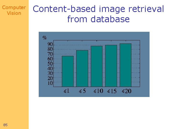
Computer Vision 85 Content-based image retrieval from database
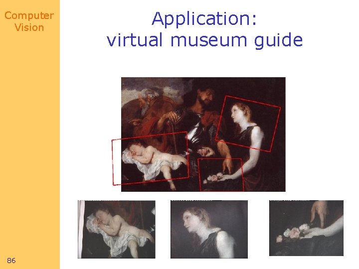
Computer Vision 86 Application: virtual museum guide
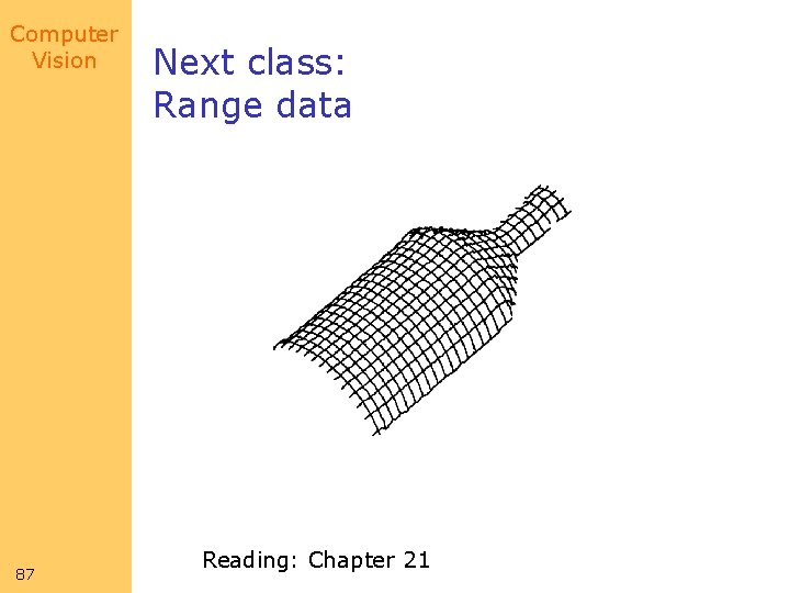
Computer Vision 87 Next class: Range data Reading: Chapter 21

Computer Vision Talk 4 pm tomorrow: Jean Ponce Three-Dimensional Computer Vision: Challenges and Opportunities Jean Ponce (ponce@cs. uiuc. edu) University of Illinois at Urbana-Champaign Ecole Normale Supirieure, Paris http: //www-cvr. ai. uiuc. edu/ponce_grp/ Abstract: This talk addresses two of the main challenges of computer vision: automatically recognizing three-dimensional (3 D) object categories in photographs despite potential within-class variations, viewpoint changes, occlusion, and clutter; and recovering accurate models of 3 D shapes observed in multiple images. I will first present a new approach to 3 D object recognition that exploits local, semi-local, and global constraints to learn visual models of texture, object, and scene categories, and identify instances of these models in photographs. I will then discuss a novel algorithm that uses the geometric and photometric constraints associated with multiple calibrated photographs to construct high-fidelity solid models of complex 3 D shapes in the form of carved visual hulls. I will conclude with a brief discussion of new application domains and wide open research issues. Joint work with Yasutaka Furukawa, Akash Kushal, Svetlana Lazebnik, Kenton Mc. Henry, Fred Rothganger, and Cordelia Schmid. 88
- Slides: 88