Computer Vision Fitting and Alignment Slides borrowed from

Computer Vision - Fitting and Alignment (Slides borrowed from various presentations)

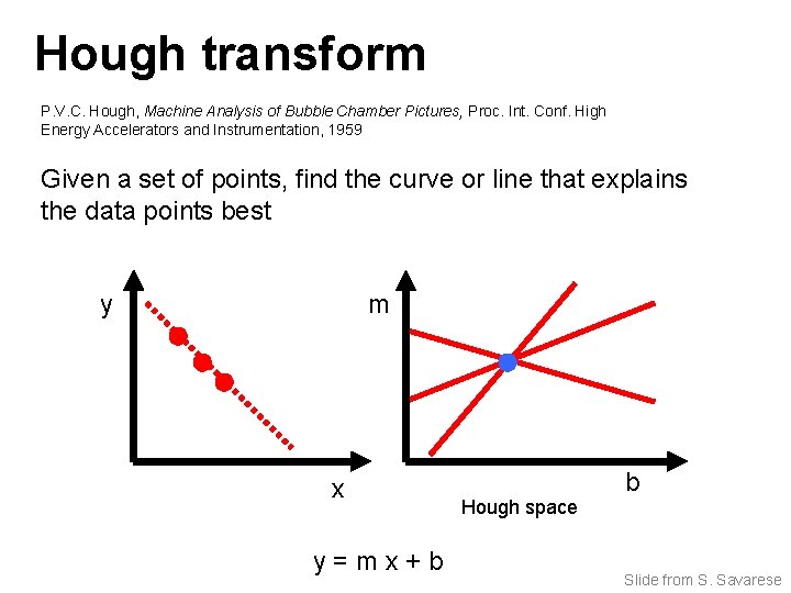
Hough transform P. V. C. Hough, Machine Analysis of Bubble Chamber Pictures, Proc. Int. Conf. High Energy Accelerators and Instrumentation, 1959 Given a set of points, find the curve or line that explains the data points best y m x y=mx+b Hough space b Slide from S. Savarese

Hough transform y m b x y m 3 x Slide from S. Savarese 5 3 3 2 2 3 7 11 10 4 3 2 1 1 0 5 3 2 3 4 1 b

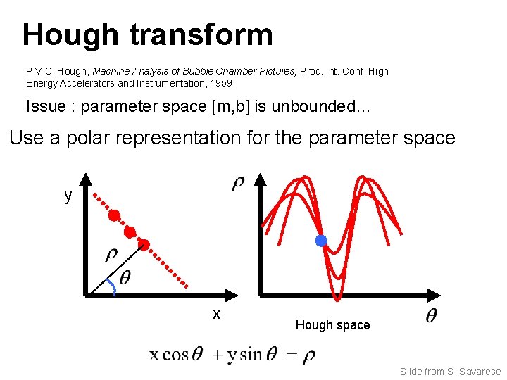
Hough transform P. V. C. Hough, Machine Analysis of Bubble Chamber Pictures, Proc. Int. Conf. High Energy Accelerators and Instrumentation, 1959 Issue : parameter space [m, b] is unbounded… Use a polar representation for the parameter space y x Hough space Slide from S. Savarese

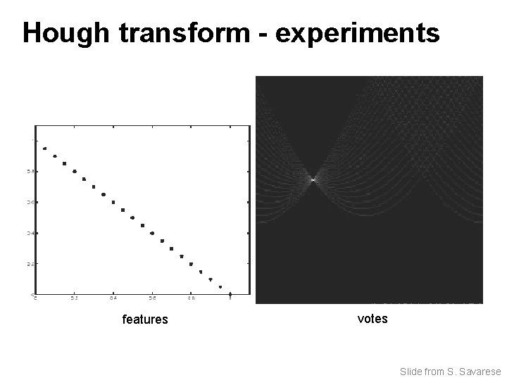
Hough transform - experiments features votes Slide from S. Savarese

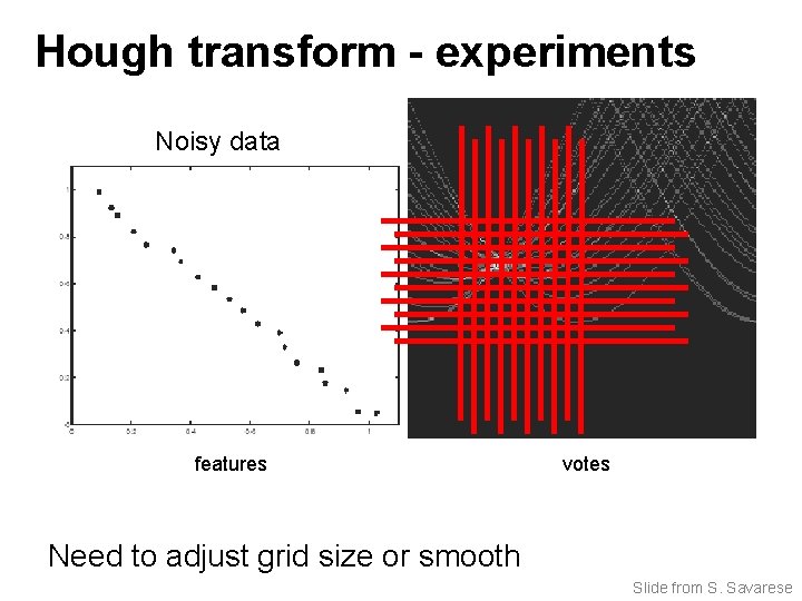
Hough transform - experiments Noisy data features votes Need to adjust grid size or smooth Slide from S. Savarese

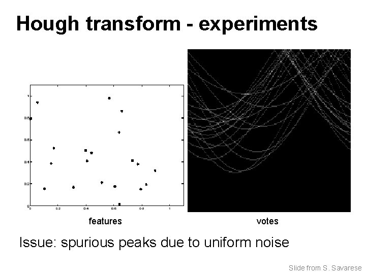
Hough transform - experiments features votes Issue: spurious peaks due to uniform noise Slide from S. Savarese

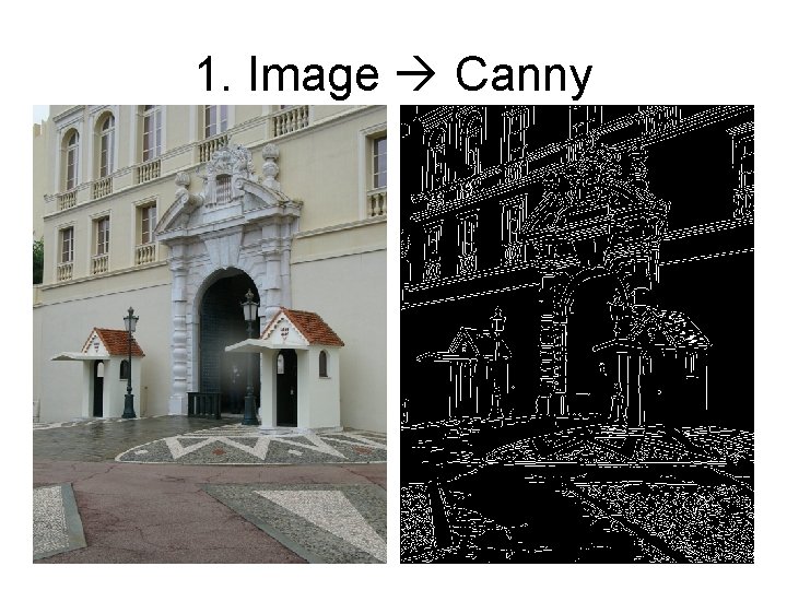
1. Image Canny

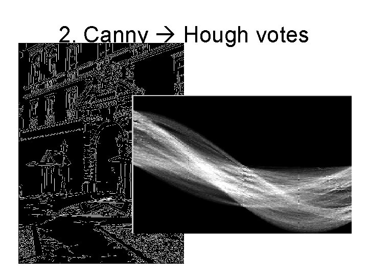
2. Canny Hough votes

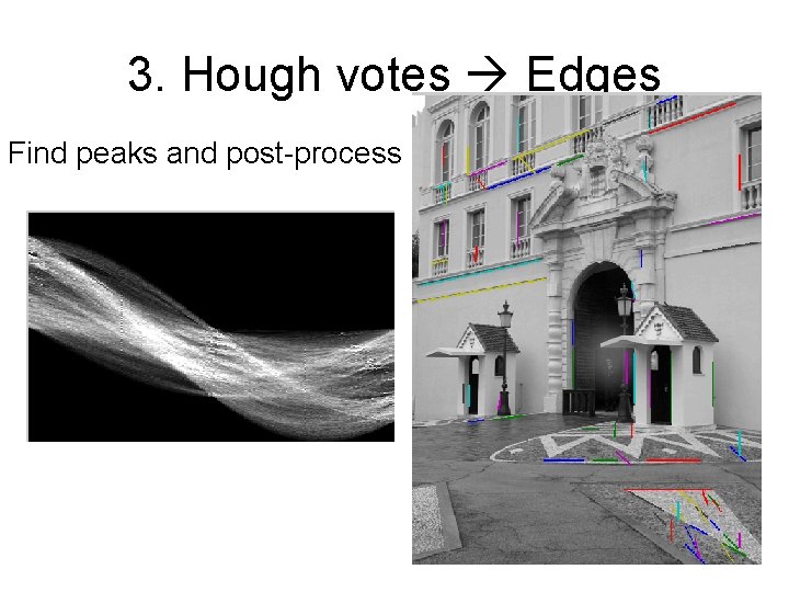
3. Hough votes Edges Find peaks and post-process

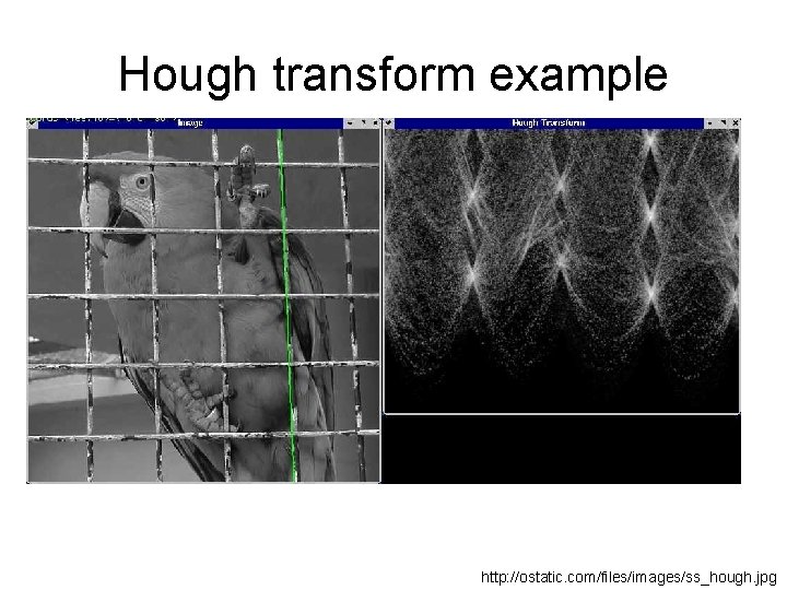
Hough transform example http: //ostatic. com/files/images/ss_hough. jpg

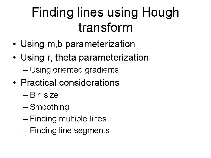
Finding lines using Hough transform • Using m, b parameterization • Using r, theta parameterization – Using oriented gradients • Practical considerations – Bin size – Smoothing – Finding multiple lines – Finding line segments

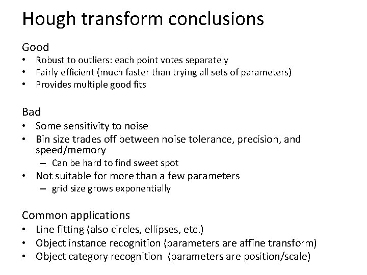
Hough transform conclusions Good • Robust to outliers: each point votes separately • Fairly efficient (much faster than trying all sets of parameters) • Provides multiple good fits Bad • Some sensitivity to noise • Bin size trades off between noise tolerance, precision, and speed/memory – Can be hard to find sweet spot • Not suitable for more than a few parameters – grid size grows exponentially Common applications • Line fitting (also circles, ellipses, etc. ) • Object instance recognition (parameters are affine transform) • Object category recognition (parameters are position/scale)

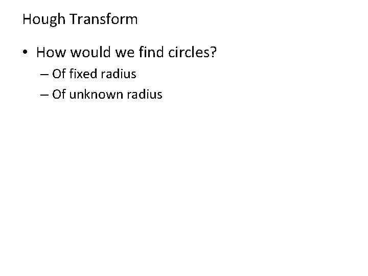
Hough Transform • How would we find circles? – Of fixed radius – Of unknown radius

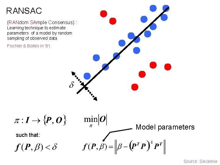
RANSAC (RANdom SAmple Consensus) : Learning technique to estimate parameters of a model by random sampling of observed data Fischler & Bolles in ‘ 81. Model parameters such that: Source: Savarese

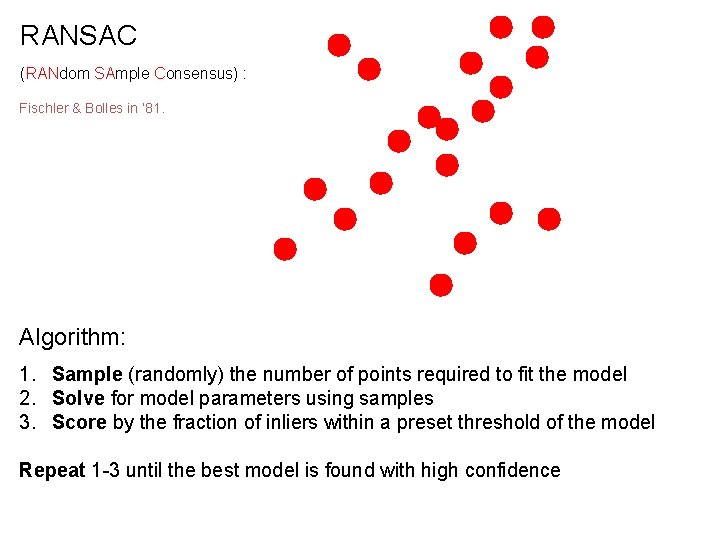
RANSAC (RANdom SAmple Consensus) : Fischler & Bolles in ‘ 81. Algorithm: 1. Sample (randomly) the number of points required to fit the model 2. Solve for model parameters using samples 3. Score by the fraction of inliers within a preset threshold of the model Repeat 1 -3 until the best model is found with high confidence

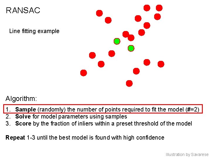
RANSAC Line fitting example Algorithm: 1. Sample (randomly) the number of points required to fit the model (#=2) 2. Solve for model parameters using samples 3. Score by the fraction of inliers within a preset threshold of the model Repeat 1 -3 until the best model is found with high confidence Illustration by Savarese

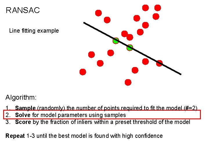
RANSAC Line fitting example Algorithm: 1. Sample (randomly) the number of points required to fit the model (#=2) 2. Solve for model parameters using samples 3. Score by the fraction of inliers within a preset threshold of the model Repeat 1 -3 until the best model is found with high confidence

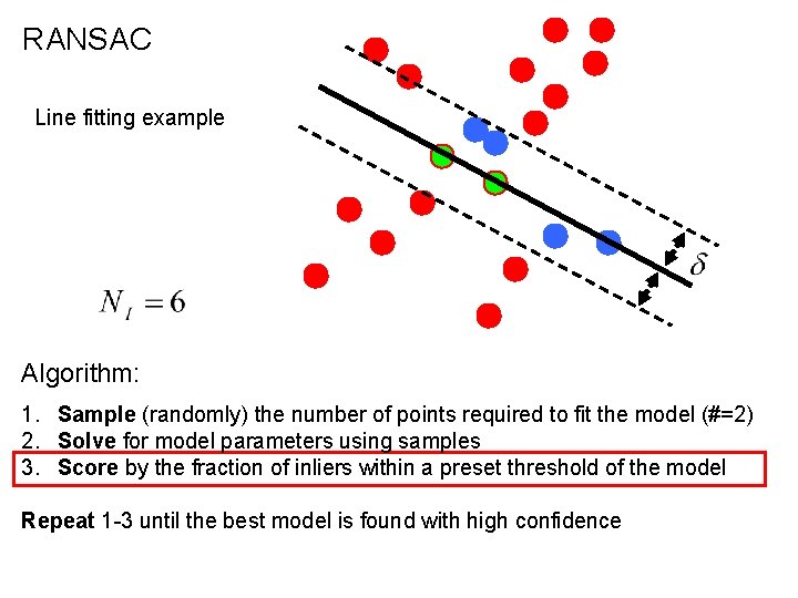
RANSAC Line fitting example Algorithm: 1. Sample (randomly) the number of points required to fit the model (#=2) 2. Solve for model parameters using samples 3. Score by the fraction of inliers within a preset threshold of the model Repeat 1 -3 until the best model is found with high confidence

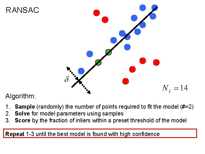
RANSAC Algorithm: 1. Sample (randomly) the number of points required to fit the model (#=2) 2. Solve for model parameters using samples 3. Score by the fraction of inliers within a preset threshold of the model Repeat 1 -3 until the best model is found with high confidence

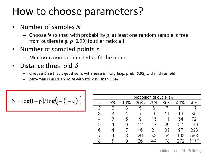
How to choose parameters? • Number of samples N – Choose N so that, with probability p, at least one random sample is free from outliers (e. g. p=0. 99) (outlier ratio: e ) • Number of sampled points s – Minimum number needed to fit the model • Distance threshold – Choose so that a good point with noise is likely (e. g. , prob=0. 95) within threshold – Zero-mean Gaussian noise with std. dev. σ: t 2=3. 84σ2 proportion of outliers e s 2 3 4 5 6 7 8 5% 2 3 3 4 4 4 5 10% 3 4 5 6 7 8 9 20% 25% 30% 40% 5 6 7 11 17 7 9 11 19 35 9 13 17 34 72 12 17 26 57 146 16 24 37 97 293 20 33 54 163 588 26 44 78 272 1177 modified from M. Pollefeys

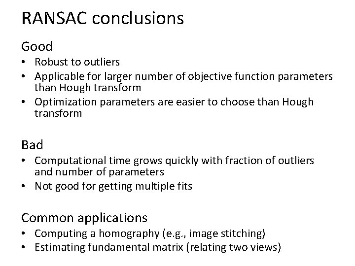
RANSAC conclusions Good • Robust to outliers • Applicable for larger number of objective function parameters than Hough transform • Optimization parameters are easier to choose than Hough transform Bad • Computational time grows quickly with fraction of outliers and number of parameters • Not good for getting multiple fits Common applications • Computing a homography (e. g. , image stitching) • Estimating fundamental matrix (relating two views)

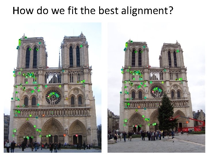
How do we fit the best alignment?

Alignment • Alignment: find parameters of model that maps one set of points to another • Typically want to solve for a global transformation that accounts for *most* true correspondences • Difficulties – Noise (typically 1 -3 pixels) – Outliers (often 50%)

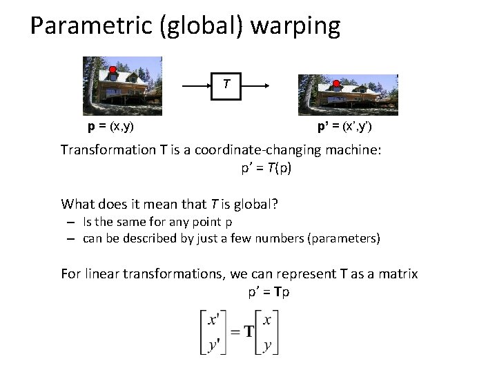
Parametric (global) warping T p = (x, y) p’ = (x’, y’) Transformation T is a coordinate-changing machine: p’ = T(p) What does it mean that T is global? – Is the same for any point p – can be described by just a few numbers (parameters) For linear transformations, we can represent T as a matrix p’ = Tp

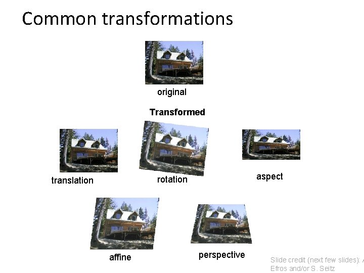
Common transformations original Transformed aspect rotation translation affine perspective Slide credit (next few slides): A Efros and/or S. Seitz

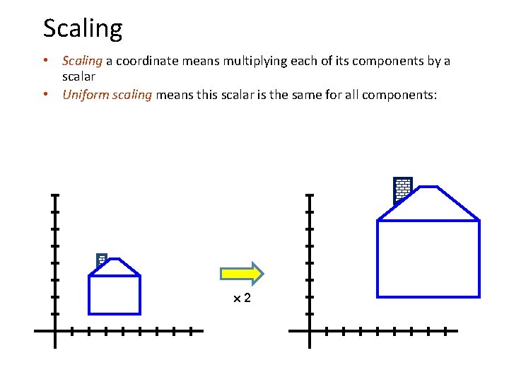
Scaling • Scaling a coordinate means multiplying each of its components by a scalar • Uniform scaling means this scalar is the same for all components: 2

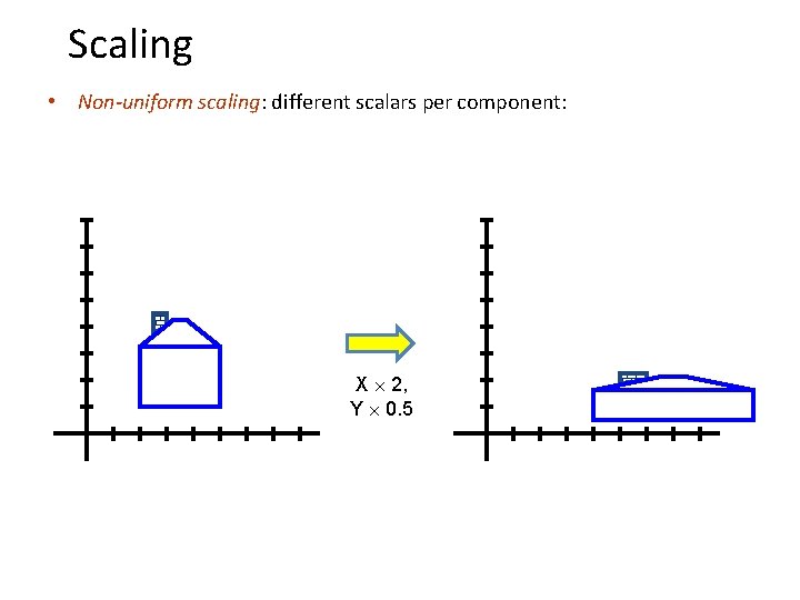
Scaling • Non-uniform scaling: different scalars per component: X 2, Y 0. 5

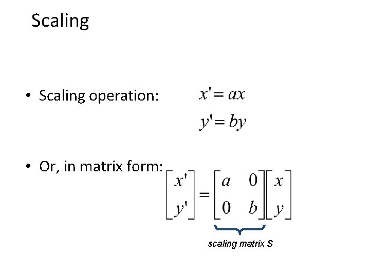
Scaling • Scaling operation: • Or, in matrix form: scaling matrix S

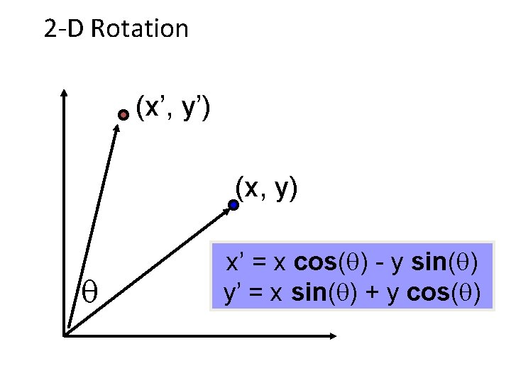
2 -D Rotation (x’, y’) (x, y) x’ = x cos( ) - y sin( ) y’ = x sin( ) + y cos( )

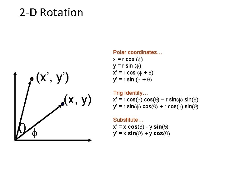
2 -D Rotation (x’, y’) (x, y) f Polar coordinates… x = r cos (f) y = r sin (f) x’ = r cos (f + ) y’ = r sin (f + ) Trig Identity… x’ = r cos(f) cos( ) – r sin(f) sin( ) y’ = r sin(f) cos( ) + r cos(f) sin( ) Substitute… x’ = x cos( ) - y sin( ) y’ = x sin( ) + y cos( )

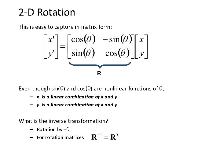
2 -D Rotation This is easy to capture in matrix form: R Even though sin( ) and cos( ) are nonlinear functions of , – x’ is a linear combination of x and y – y’ is a linear combination of x and y What is the inverse transformation? – Rotation by – – For rotation matrices

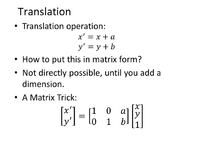
Translation •

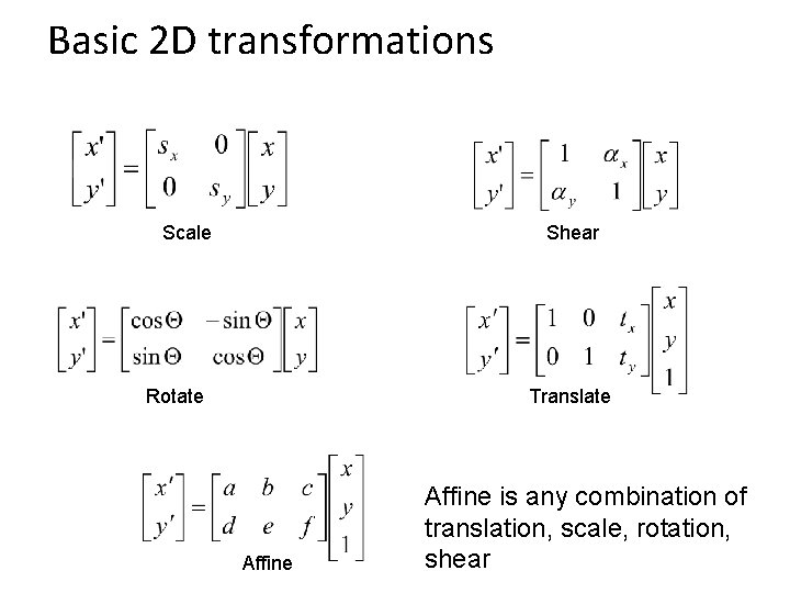
Basic 2 D transformations Scale Shear Rotate Translate Affine is any combination of translation, scale, rotation, shear

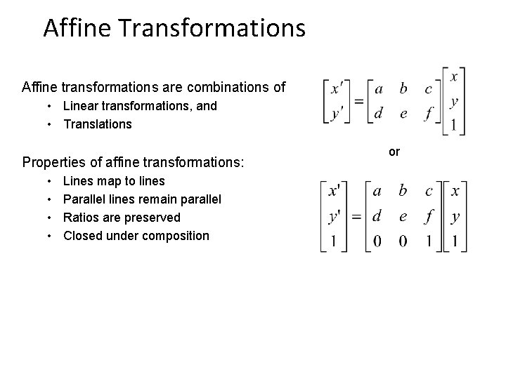
Affine Transformations Affine transformations are combinations of • Linear transformations, and • Translations Properties of affine transformations: • • Lines map to lines Parallel lines remain parallel Ratios are preserved Closed under composition or

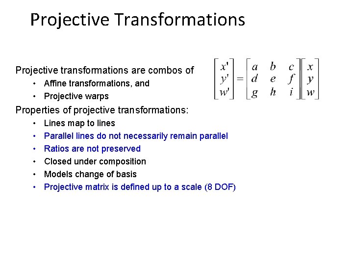
Projective Transformations Projective transformations are combos of • Affine transformations, and • Projective warps Properties of projective transformations: • • • Lines map to lines Parallel lines do not necessarily remain parallel Ratios are not preserved Closed under composition Models change of basis Projective matrix is defined up to a scale (8 DOF)

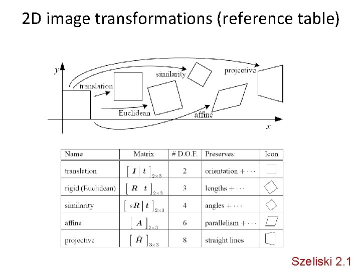
2 D image transformations (reference table) Szeliski 2. 1

Example: solving for translation A 1 A 2 A 3 B 1 B 2 B 3 Given matched points in {A} and {B}, estimate the translation of the object

Example: solving for translation A 1 A 2 A 3 (tx, ty) B 1 B 2 Least squares solution 1. Write down objective function 2. Derived solution a) Compute derivative b) Compute solution 3. Computational solution a) Write in form Ax=b b) Solve using pseudo-inverse or eigenvalue decomposition B 3

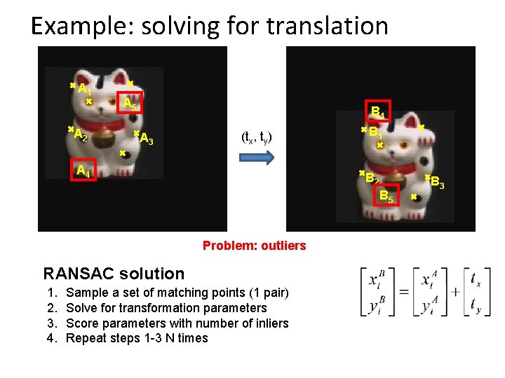
Example: solving for translation A 1 A 2 A 5 B 4 A 3 (tx, ty) A 4 B 1 B 2 B 5 Problem: outliers RANSAC solution 1. 2. 3. 4. Sample a set of matching points (1 pair) Solve for transformation parameters Score parameters with number of inliers Repeat steps 1 -3 N times B 3

RANSAC for Image Matching (Detailed) 1. Detect features in each image (eg. , use blob detection). 2. Randomly select enough matches to determine a transformation that will align the images. 3. –Eg. , if we use an affine transformation, we need 3 matching points. Pick three random points in image one, and match each to a random point in image 2. O(n 6) possible matches. 4. Apply this transformation to all points in image 1. 5. Count number of points that are transformed “near” (say within 2 pixels) of a point in image 2. 6. Pick transformation that matches the most points.

Improvements • Problem: O(n 6) matches is a lot. Only one in O(n 3) will be right. • Solution: for each point in image 1, use SIFT descriptors to find point in image 2 that provides best match. • If most of these matches are correct, we now have much higher chance of finding good matches, with a small chance that we miss some.

Example: solving for translation B 4 A 1 A 2 B 5 (tx, ty) A 3 B 1 B 2 A 4 A 5 B 6 B 3 A 6 Problem: outliers, multiple objects, and/or many-to-one matches Hough transform solution 1. Initialize a grid of parameter values 2. Each matched pair casts a vote for consistent values 3. Find the parameters with the most votes 4. Solve using least squares with inliers

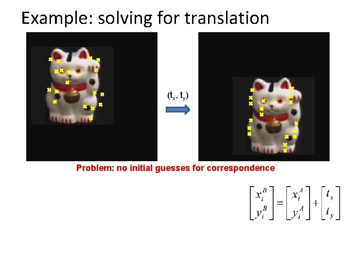
Example: solving for translation (tx, ty) Problem: no initial guesses for correspondence

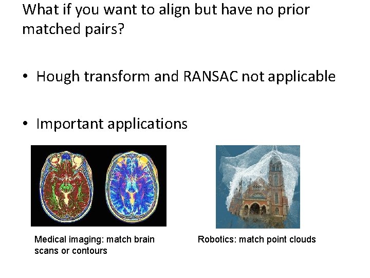
What if you want to align but have no prior matched pairs? • Hough transform and RANSAC not applicable • Important applications Medical imaging: match brain scans or contours Robotics: match point clouds

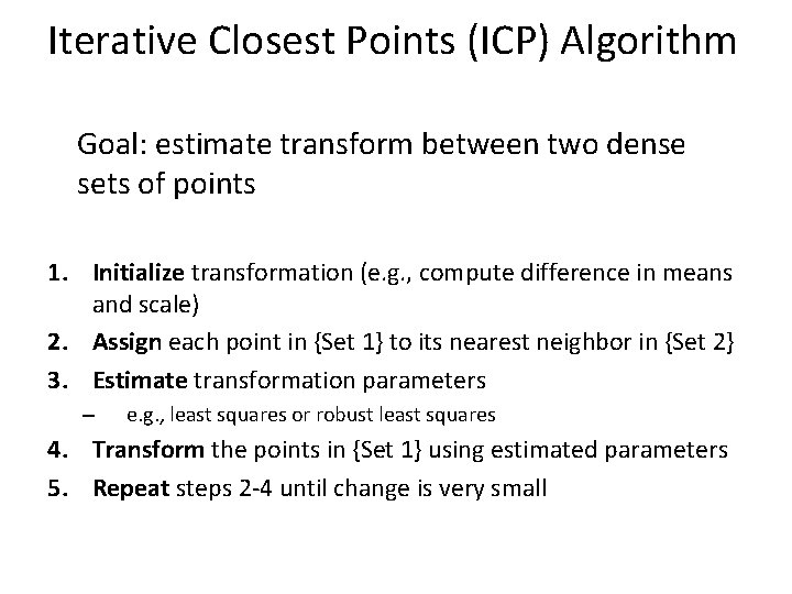
Iterative Closest Points (ICP) Algorithm Goal: estimate transform between two dense sets of points 1. Initialize transformation (e. g. , compute difference in means and scale) 2. Assign each point in {Set 1} to its nearest neighbor in {Set 2} 3. Estimate transformation parameters – e. g. , least squares or robust least squares 4. Transform the points in {Set 1} using estimated parameters 5. Repeat steps 2 -4 until change is very small

Example: solving for translation (tx, ty) Problem: no initial guesses for correspondence ICP solution 1. 2. 3. 4. Find nearest neighbors for each point Compute transform using matches Move points using transform Repeat steps 1 -3 until convergence

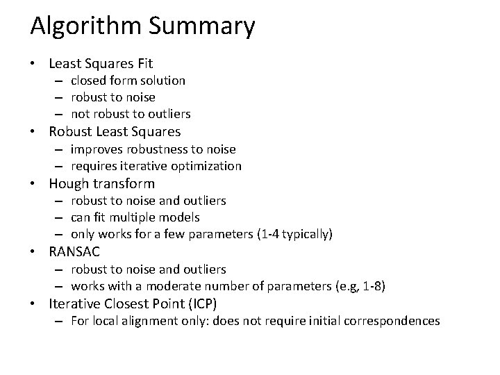
Algorithm Summary • Least Squares Fit – closed form solution – robust to noise – not robust to outliers • Robust Least Squares – improves robustness to noise – requires iterative optimization • Hough transform – robust to noise and outliers – can fit multiple models – only works for a few parameters (1 -4 typically) • RANSAC – robust to noise and outliers – works with a moderate number of parameters (e. g, 1 -8) • Iterative Closest Point (ICP) – For local alignment only: does not require initial correspondences