Computer Sciences Department 1 binary tree Properties Heap

Computer Sciences Department 1

binary tree (Properties) Heap tree (Properties) Property 1: each node can have up to two successor nodes (children) The predecessor node of a node is called its parent The "beginning" node is called the root (no parent) A node without children is called a leaf Property 2: a unique path exists from the root to every other node + max-heap or min-heap property Computer Sciences Department 3

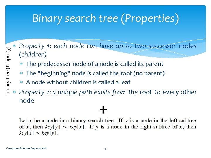
binary tree (Property) Binary search tree (Properties) Property 1: each node can have up to two successor nodes (children) The predecessor node of a node is called its parent The "beginning" node is called the root (no parent) A node without children is called a leaf Property 2: a unique path exists from the root to every other node + Computer Sciences Department 4

Advanced Design and Analysis Techniques (15. 1, 15. 2, 15. 3 , 15. 4 and 15. 5) Computer Sciences Department 5

Objectives Problem Formulation Examples The Basic Problem Principle of optimality Important techniques: dynamic programming (Chapter 15), greedy algorithms (Chapter 16) Computer Sciences Department 6

Techniques -1 This part covers three important techniques for the design and analysis of efficient algorithms: dynamic programming (Chapter 15), greedy algorithms (Chapter 16) Computer Sciences Department 7

Techniques - 2 Earlier parts have presented other widely applicable techniques, such as divide-and-conquer, randomization, and the solution of recurrences. Computer Sciences Department 8

Dynamic programming is an optimization approach that transforms a complex problem into a sequence of simpler problems. It is used in many areas such as Computer science “theory, graphics, AI, systems, …. etc” Dynamic programming typically applies to optimization problems in which a set of choices must be made in order to arrive at an optimal solution. Dynamic programming is effective when a given subproblem may arise from more than one partial set of choices; the key technique is to store the solution to each subproblem in case it should reappear. Computer Sciences Department 9

Greedy algorithms Like dynamic-programming algorithms, greedy algorithms typically apply to optimization problems in which a set of choices must be made in order to arrive at an optimal solution. The idea of a greedy algorithm is to make each choice in a locally optimal manner. Computer Sciences Department 10

Dynamic programming -1 Dynamic programming, like the divide-and-conquer method, solves problems by combining the solutions to subproblems. Divide and- conquer algorithms partition the problem into independent subproblems, solve the subproblems recursively, and then combine their solutions to solve the original problem. Computer Sciences Department 11

Dynamic programming -2 Dynamic programming is applicable when the subproblems are not independent, that is, when subproblems share subsubproblems. A dynamic-programming algorithm solves every subsubproblem just once and then saves its answer in a table, thereby avoiding the work of recomputing the answer every time the subsubproblem is encountered. Computer Sciences Department 12

Dynamic programming -2 Dynamic programming is typically applied to optimization problems. In such problems there can be many possible solutions. Each solution has a value, and we wish to find a solution with the optimal (minimum or maximum) value. We call such a solution an optimal solution to the problem, as opposed to the optimal solution, since there may be several solutions that achieve the optimal value. Computer Sciences Department 13

The development of a dynamicprogramming algorithm The development of a dynamic-programming algorithm can be broken into a sequence of four steps. 1. Characterize the structure of an optimal solution. 2. Recursively define the value of an optimal solution. 3. Compute the value of an optimal solution in a bottom-up fashion. 4. Construct an optimal solution from computed information. Computer Sciences Department 14

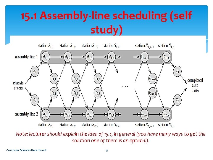
15. 1 Assembly-line scheduling (self study) Note: lecturer should explain the idea of 15. 1, in general (you have many ways to get the solution one of them is an optimal). Computer Sciences Department 15

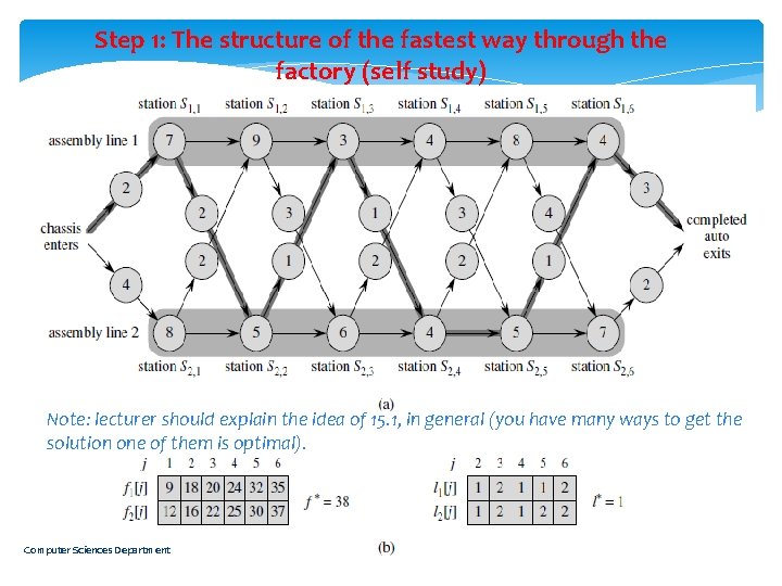
Step 1: The structure of the fastest way through the factory (self study) Note: lecturer should explain the idea of 15. 1, in general (you have many ways to get the solution one of them is optimal). Computer Sciences Department 16

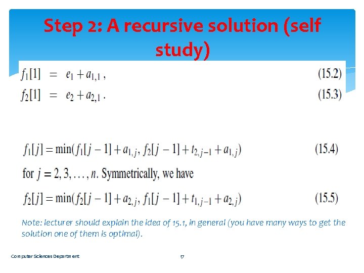
Step 2: A recursive solution (self study) Note: lecturer should explain the idea of 15. 1, in general (you have many ways to get the solution one of them is optimal). Computer Sciences Department 17

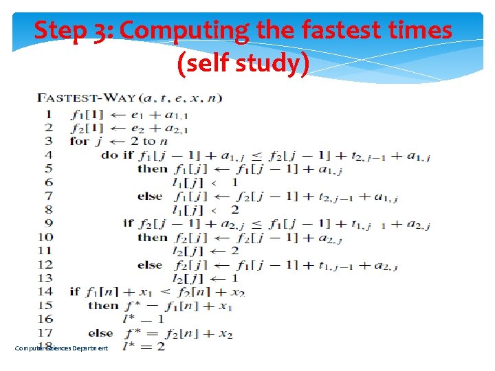
Step 3: Computing the fastest times (self study) Computer Sciences Department 18

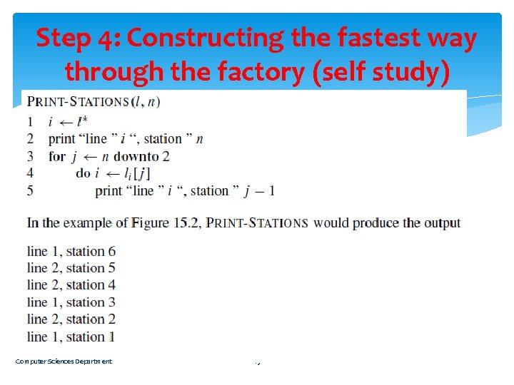
Step 4: Constructing the fastest way through the factory (self study) Computer Sciences Department 19

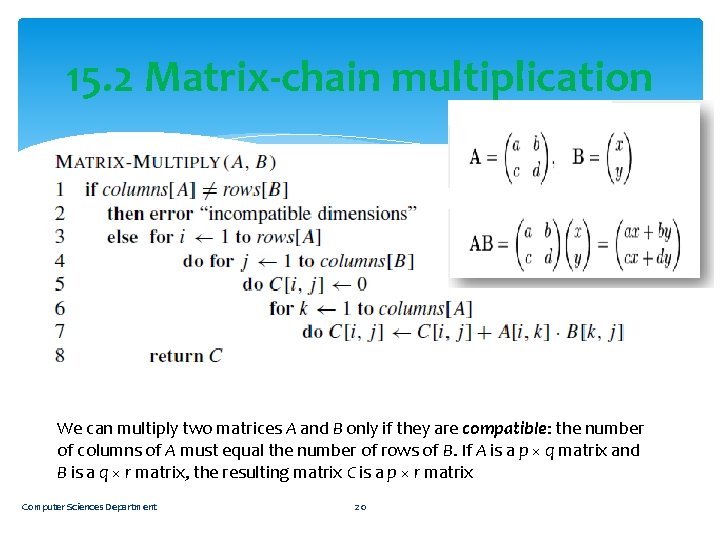
15. 2 Matrix-chain multiplication We can multiply two matrices A and B only if they are compatible: the number of columns of A must equal the number of rows of B. If A is a p × q matrix and B is a q × r matrix, the resulting matrix C is a p × r matrix Computer Sciences Department 20

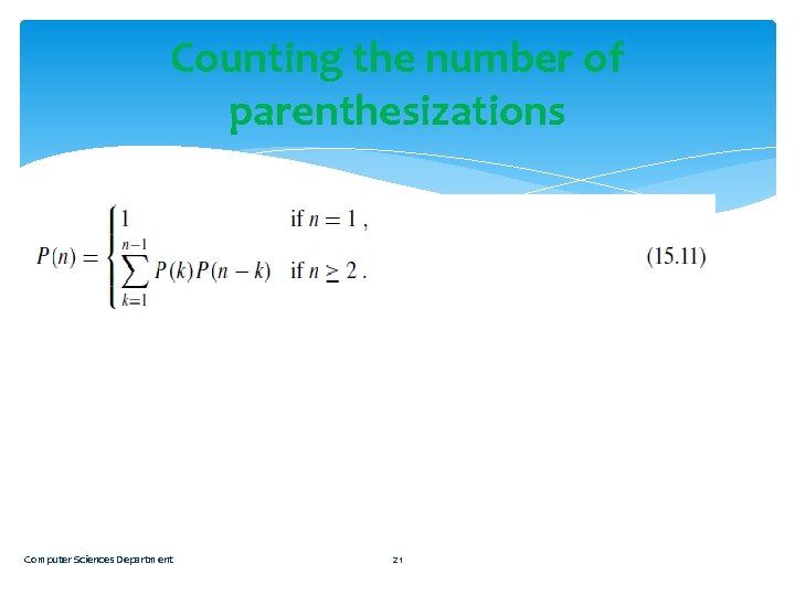
Counting the number of parenthesizations Computer Sciences Department 21

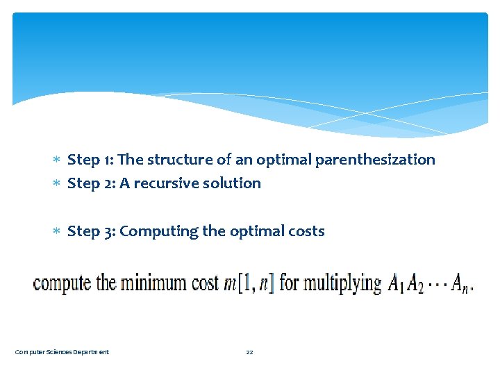
Step 1: The structure of an optimal parenthesization Step 2: A recursive solution Step 3: Computing the optimal costs Computer Sciences Department 22

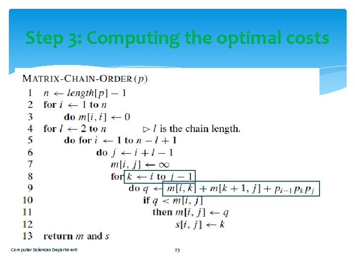
Step 3: Computing the optimal costs Computer Sciences Department 23

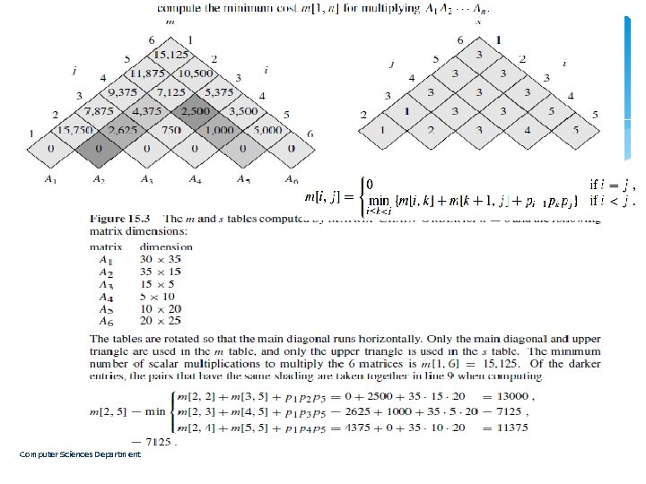
Computer Sciences Department 24

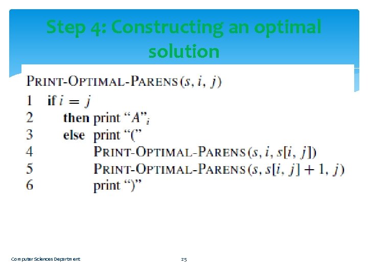
Step 4: Constructing an optimal solution Computer Sciences Department 25

Step 4 (explanation) Computer Sciences Department 26

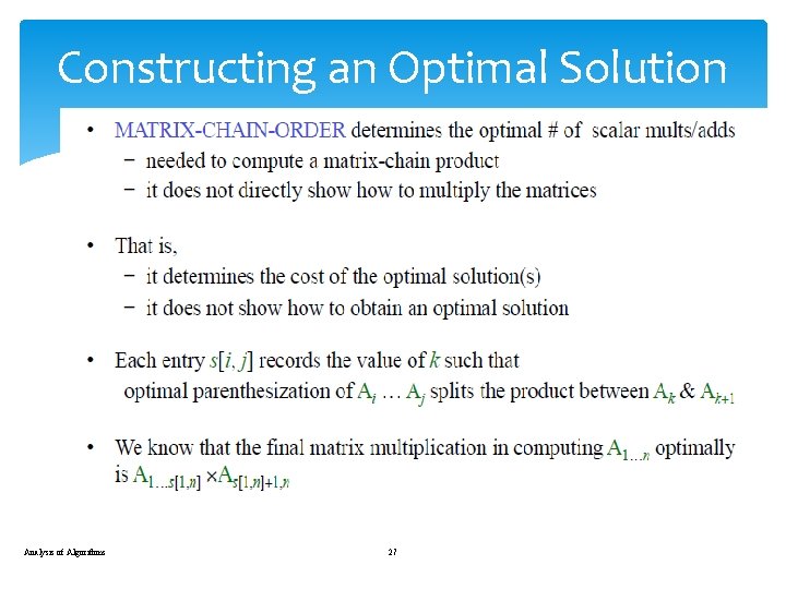
Constructing an Optimal Solution Analysis of Algorithms 27

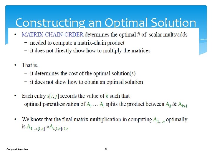
Constructing an Optimal Solution Analysis of Algorithms 28

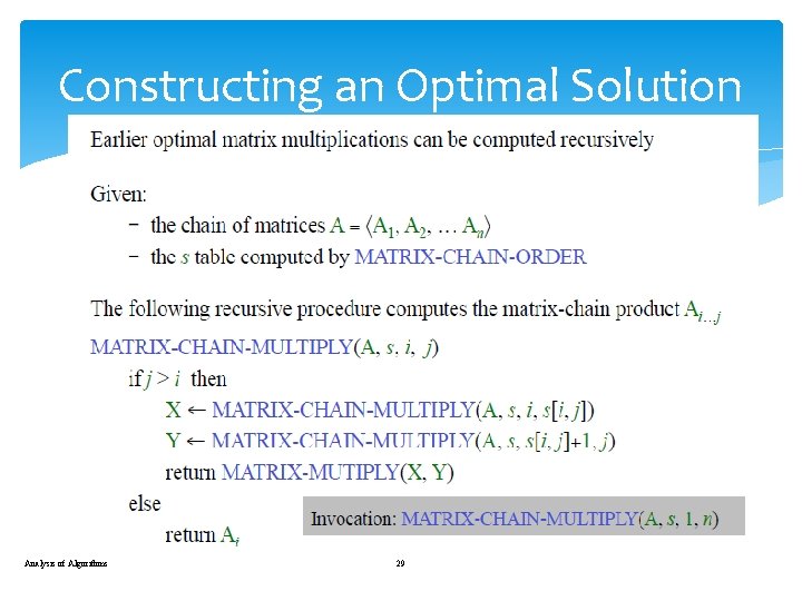
Constructing an Optimal Solution Analysis of Algorithms 29

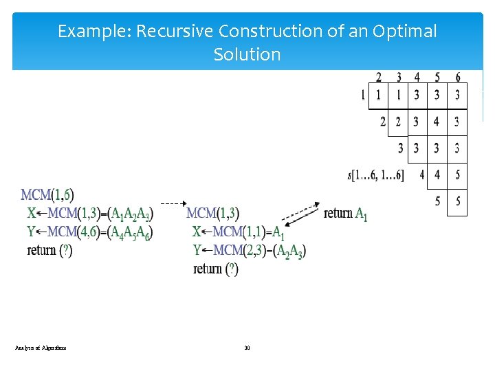
Example: Recursive Construction of an Optimal Solution Analysis of Algorithms 30

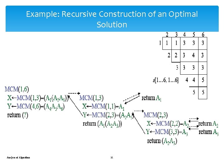
Example: Recursive Construction of an Optimal Solution Analysis of Algorithms 31

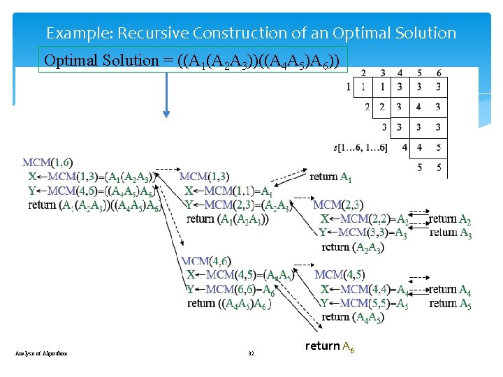
Example: Recursive Construction of an Optimal Solution = ((A 1(A 2 A 3))((A 4 A 5)A 6)) Analysis of Algorithms 32 return A 6

Elements of dynamic programming (self stady) 15. 3 Computer Sciences Department 33

Optimal substructure The first step in solving an optimization problem by dynamic programming is to characterize the structure of an optimal solution. Recall that a problem exhibits optimal substructure if an optimal solution to the problem contains within it optimal solutions to subproblems. Computer Sciences Department 34

Characterize the space of subproblems a good rule of thumb is to try to keep the space as simple as possible, and then to expand it as necessary. For example: the space of subproblems that we considered for assembly-line scheduling was the fastest way from entry into the factory through stations S 1, j and S 2, j. This subproblem space worked well, and there was no need to try a more general space of subproblems. Computer Sciences Department 35

Optimal substructure varies across problem domains in two ways: 1. how many subproblems are used in an optimal solution to the original problem, and 2. how many choices we have in determining which subproblem(s) to use in an optimal solution. Computer Sciences Department 36

Assembly-line scheduling In assembly-line scheduling, an optimal solution uses just one subproblem, but we must consider two choices in order to determine an optimal solution. To find the fastest way through station Si, j, we use either the fastest way through S 1, j− 1 or the fastest way through S 2, j− 1; whichever we use represents the one subproblem that we must optimally solve. Computer Sciences Department 37

Running time of a dynamicprogramming Informally, the running time of a dynamicprogramming algorithm depends on the product of two factors: the number of subproblems overall and how many choices we look at for each subproblem. In assembly-line scheduling, we had Theta (n) subproblems overall, and only two choices to examine for each, yielding a Theta (n) running time. Computer Sciences Department 38

Be careful One should be careful not to assume that optimal substructure applies when it does not. Unweighted shortest path: 2 Find a path from u to v consisting of the fewest edges. Such a path must be simple, since removing a cycle from a path produces a path with fewer edges. Unweighted longest simple path: Find a simple path from u to v consisting of the most edges. We need to include the requirement of simplicity because otherwise we can traverse a cycle as many times as we like to create paths with an arbitrarily large number of edges. A path is called simple if it does not have any repeated vertices. Computer Sciences Department 39

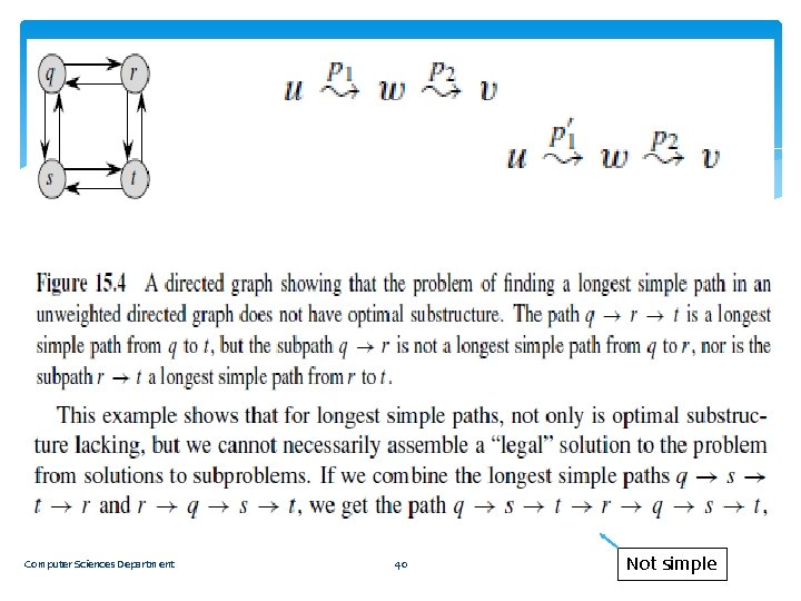
Computer Sciences Department 40 Not simple

read only Overlapping subproblems Reconstructing an optimal solution Memoization 15. 4 Longest common subsequence Computer Sciences Department 41

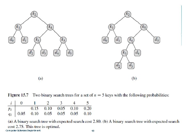
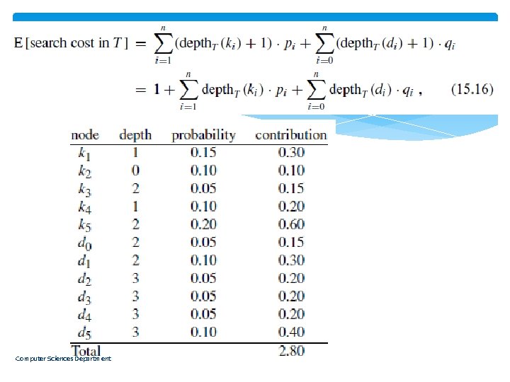
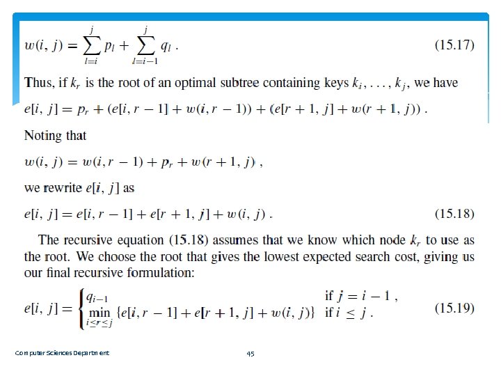
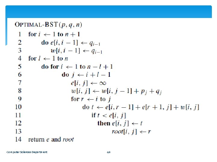
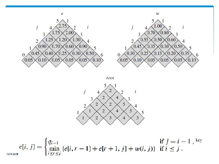
15. 5 Optimal binary search trees Suppose that we are designing a program to translate text from English to French. For each occurrence of each English word in the text, we need to look up its French equivalent. One way to perform these lookup operations is to build a binary search tree with n English words as keys and French equivalents as satellite data. Computer Sciences Department 42

Computer Sciences Department 43

Computer Sciences Department 44

Computer Sciences Department 45

Computer Sciences Department 46

Computer Sciences Department 47

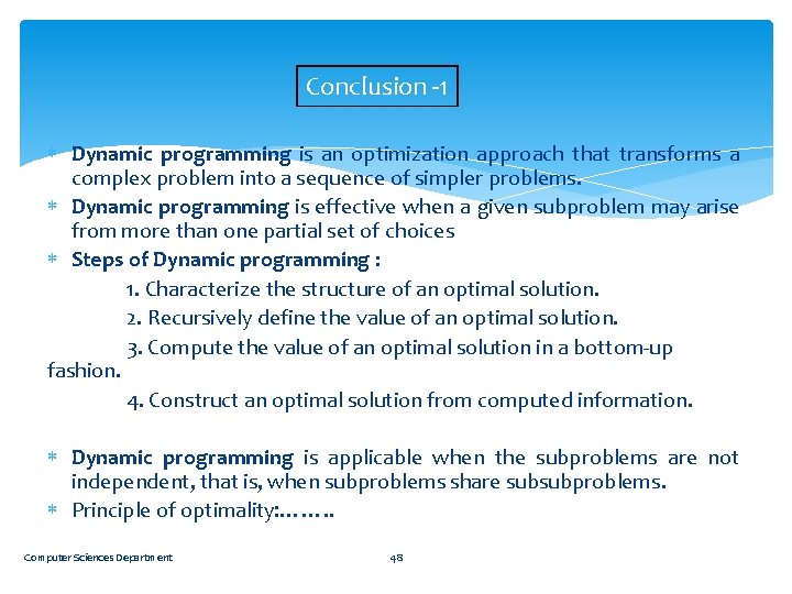
Conclusion -1 Dynamic programming is an optimization approach that transforms a complex problem into a sequence of simpler problems. Dynamic programming is effective when a given subproblem may arise from more than one partial set of choices Steps of Dynamic programming : 1. Characterize the structure of an optimal solution. 2. Recursively define the value of an optimal solution. 3. Compute the value of an optimal solution in a bottom-up fashion. 4. Construct an optimal solution from computed information. Dynamic programming is applicable when the subproblems are not independent, that is, when subproblems share subsubproblems. Principle of optimality: ……. . Computer Sciences Department 48