Computer Organization and Architecture Designing for Performance 11

Computer Organization and Architecture Designing for Performance 11 th Edition Chapter 2 Performance Concepts Copyright © 2019, 2016, 2013 Pearson Education, Inc. All Rights Reserved

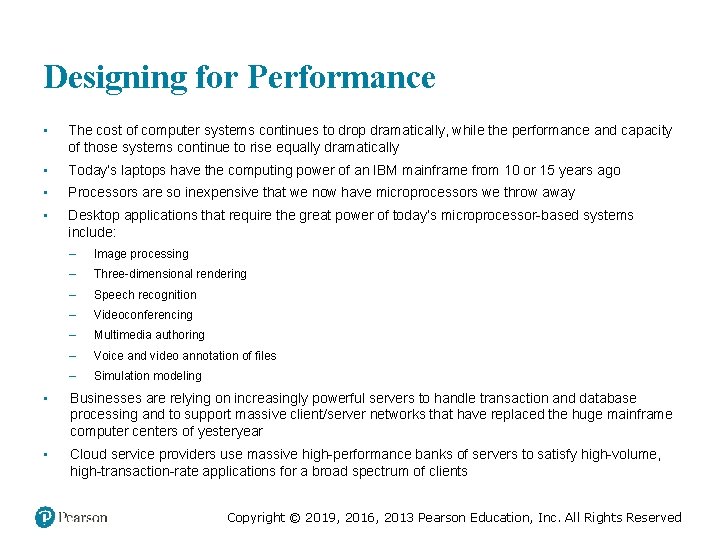
Designing for Performance • The cost of computer systems continues to drop dramatically, while the performance and capacity of those systems continue to rise equally dramatically • Today’s laptops have the computing power of an IBM mainframe from 10 or 15 years ago • Processors are so inexpensive that we now have microprocessors we throw away • Desktop applications that require the great power of today’s microprocessor-based systems include: – Image processing – Three-dimensional rendering – Speech recognition – Videoconferencing – Multimedia authoring – Voice and video annotation of files – Simulation modeling • Businesses are relying on increasingly powerful servers to handle transaction and database processing and to support massive client/server networks that have replaced the huge mainframe computer centers of yesteryear • Cloud service providers use massive high-performance banks of servers to satisfy high-volume, high-transaction-rate applications for a broad spectrum of clients Copyright © 2019, 2016, 2013 Pearson Education, Inc. All Rights Reserved

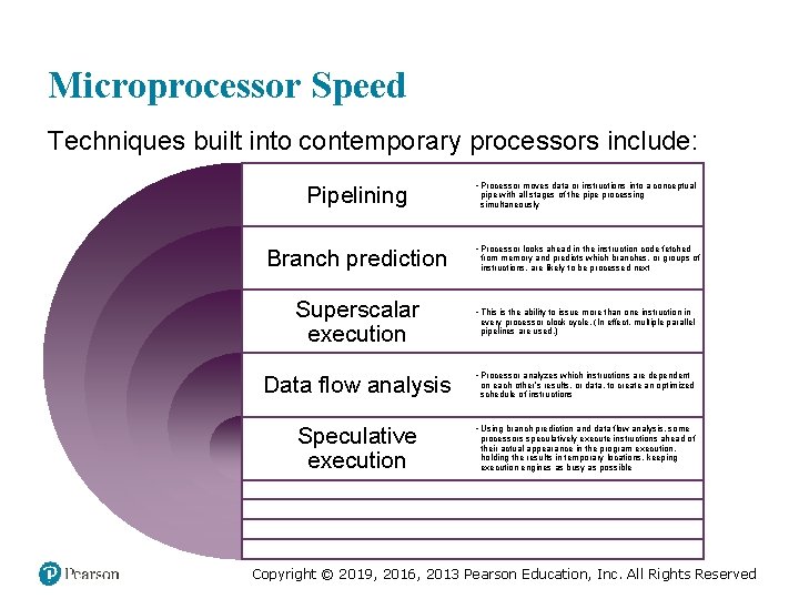
Microprocessor Speed Techniques built into contemporary processors include: Pipelining • Processor moves data or instructions into a conceptual Branch prediction • Processor looks ahead in the instruction code fetched Superscalar execution pipe with all stages of the pipe processing simultaneously from memory and predicts which branches, or groups of instructions, are likely to be processed next • This is the ability to issue more than one instruction in every processor clock cycle. (In effect, multiple parallel pipelines are used. ) Data flow analysis • Processor analyzes which instructions are dependent Speculative execution • Using branch prediction and data flow analysis, some on each other’s results, or data, to create an optimized schedule of instructions processors speculatively execute instructions ahead of their actual appearance in the program execution, holding the results in temporary locations, keeping execution engines as busy as possible Copyright © 2019, 2016, 2013 Pearson Education, Inc. All Rights Reserved

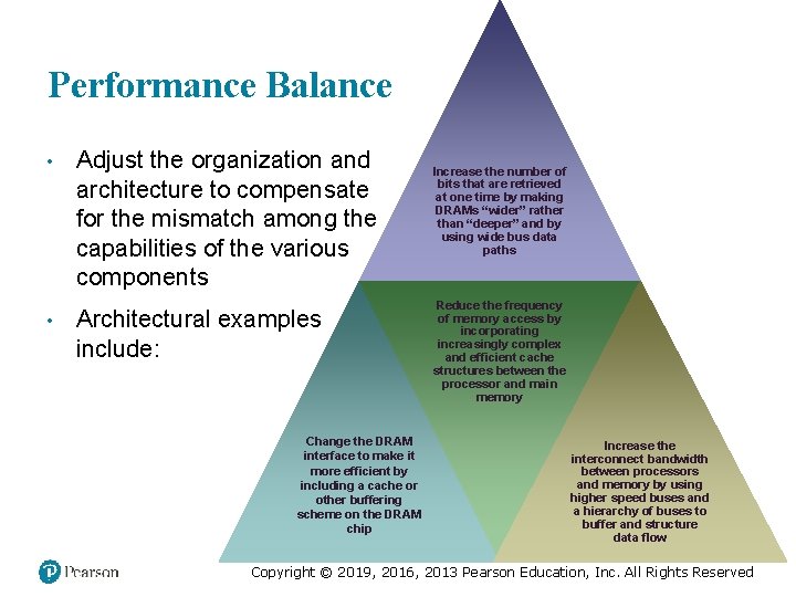
Performance Balance • • Adjust the organization and architecture to compensate for the mismatch among the capabilities of the various components Architectural examples include: Change the DRAM interface to make it more efficient by including a cache or other buffering scheme on the DRAM chip Increase the number of bits that are retrieved at one time by making DRAMs “wider” rather than “deeper” and by using wide bus data paths Reduce the frequency of memory access by incorporating increasingly complex and efficient cache structures between the processor and main memory Increase the interconnect bandwidth between processors and memory by using higher speed buses and a hierarchy of buses to buffer and structure data flow Copyright © 2019, 2016, 2013 Pearson Education, Inc. All Rights Reserved

Figure 2. 1 Copyright © 2019, 2016, 2013 Pearson Education, Inc. All Rights Reserved

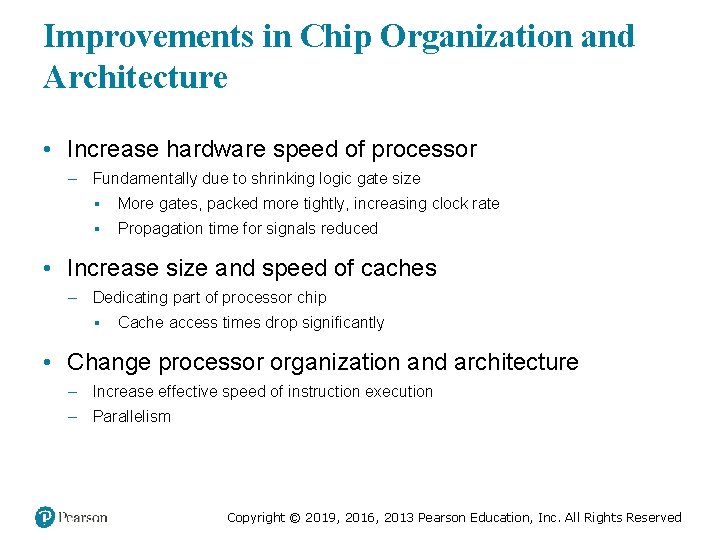
Improvements in Chip Organization and Architecture • Increase hardware speed of processor – Fundamentally due to shrinking logic gate size ▪ More gates, packed more tightly, increasing clock rate ▪ Propagation time for signals reduced • Increase size and speed of caches – Dedicating part of processor chip ▪ Cache access times drop significantly • Change processor organization and architecture – Increase effective speed of instruction execution – Parallelism Copyright © 2019, 2016, 2013 Pearson Education, Inc. All Rights Reserved

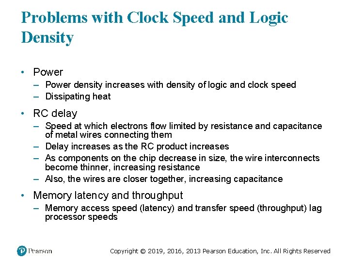
Problems with Clock Speed and Logic Density • Power – Power density increases with density of logic and clock speed – Dissipating heat • RC delay – Speed at which electrons flow limited by resistance and capacitance of metal wires connecting them – Delay increases as the RC product increases – As components on the chip decrease in size, the wire interconnects become thinner, increasing resistance – Also, the wires are closer together, increasing capacitance • Memory latency and throughput – Memory access speed (latency) and transfer speed (throughput) lag processor speeds Copyright © 2019, 2016, 2013 Pearson Education, Inc. All Rights Reserved

Figure 2. 2 Copyright © 2019, 2016, 2013 Pearson Education, Inc. All Rights Reserved

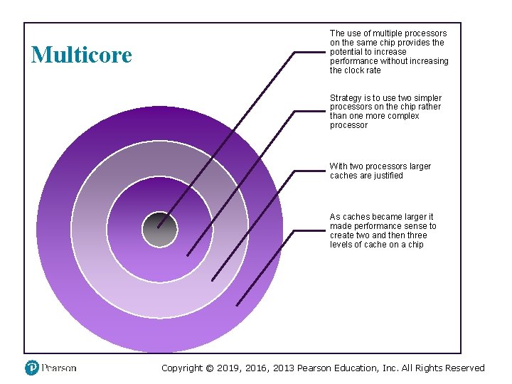
Multicore The use of multiple processors on the same chip provides the potential to increase performance without increasing the clock rate Strategy is to use two simpler processors on the chip rather than one more complex processor With two processors larger caches are justified As caches became larger it made performance sense to create two and then three levels of cache on a chip Copyright © 2019, 2016, 2013 Pearson Education, Inc. All Rights Reserved

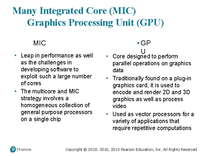
Many Integrated Core (MIC) Graphics Processing Unit (GPU) MIC • Leap in performance as well as the challenges in developing software to exploit such a large number of cores • The multicore and MIC strategy involves a homogeneous collection of general purpose processors on a single chip • GP U • Core designed to perform parallel operations on graphics data • Traditionally found on a plug-in graphics card, it is used to encode and render 2 D and 3 D graphics as well as process video • Used as vector processors for a variety of applications that require repetitive computations Copyright © 2019, 2016, 2013 Pearson Education, Inc. All Rights Reserved

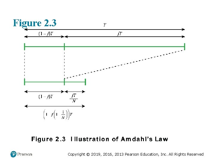
Amdahl’s Law • Gene Amdahl • Deals with the potential speedup of a program using multiple processors compared to a single processor • Illustrates the problems facing industry in the development of multi-core machines – Software must be adapted to a highly parallel execution environment to exploit the power of parallel processing • Can be generalized to evaluate and design technical improvement in a computer system Copyright © 2019, 2016, 2013 Pearson Education, Inc. All Rights Reserved

Figure 2. 3 Copyright © 2019, 2016, 2013 Pearson Education, Inc. All Rights Reserved

Figure 2. 4 Copyright © 2019, 2016, 2013 Pearson Education, Inc. All Rights Reserved

Little’s Law • Fundamental and simple relation with broad applications • Can be applied to almost any system that is statistically in steady state, and in which there is no leakage • Queuing system – If server is idle an item is served immediately, otherwise an arriving item joins a queue – There can be a single queue for a single server or for multiple servers, or multiple queues with one being for each of multiple servers • Average number of items in a queuing system equals the average rate at which items arrive multiplied by the time that an item spends in the system – Relationship requires very few assumptions – Because of its simplicity and generality it is extremely useful Copyright © 2019, 2016, 2013 Pearson Education, Inc. All Rights Reserved

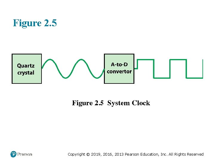
Figure 2. 5 Copyright © 2019, 2016, 2013 Pearson Education, Inc. All Rights Reserved

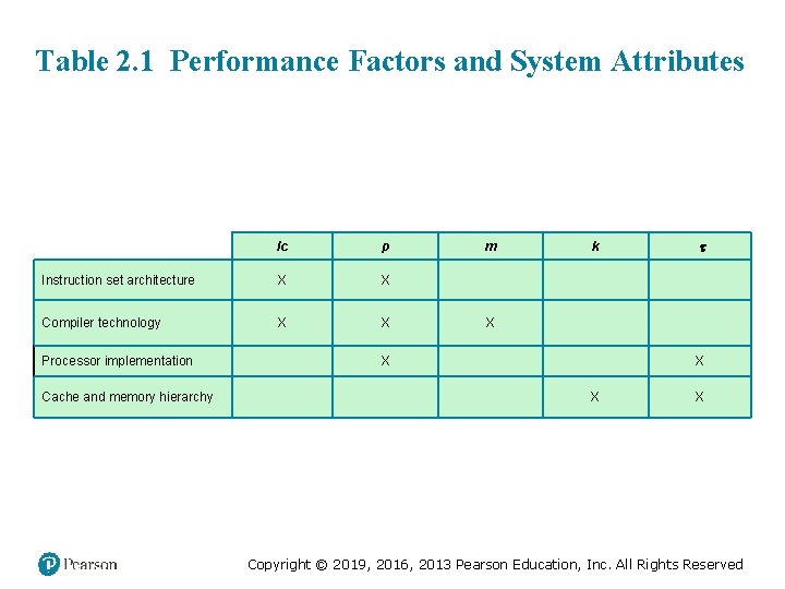
Table 2. 1 Performance Factors and System Attributes Ic p Instruction set architecture X X Compiler technology X X Processor implementation Cache and memory hierarchy m k X X X Copyright © 2019, 2016, 2013 Pearson Education, Inc. All Rights Reserved

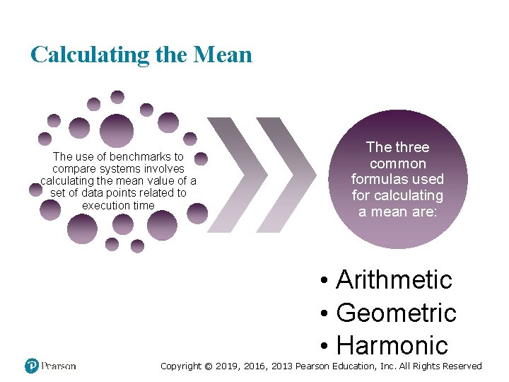
Calculating the Mean The use of benchmarks to compare systems involves calculating the mean value of a set of data points related to execution time The three common formulas used for calculating a mean are: • Arithmetic • Geometric • Harmonic Copyright © 2019, 2016, 2013 Pearson Education, Inc. All Rights Reserved

Figure 2. 6 Copyright © 2019, 2016, 2013 Pearson Education, Inc. All Rights Reserved

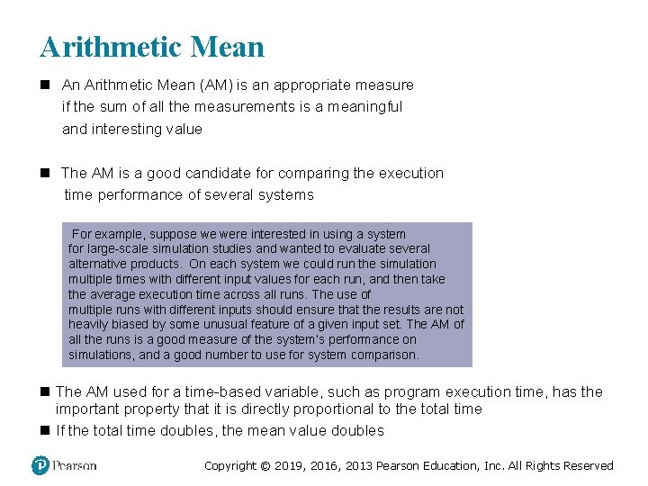
Arithmetic Mean n An Arithmetic Mean (AM) is an appropriate measure if the sum of all the measurements is a meaningful and interesting value n The AM is a good candidate for comparing the execution time performance of several systems For example, suppose we were interested in using a system for large-scale simulation studies and wanted to evaluate several alternative products. On each system we could run the simulation multiple times with different input values for each run, and then take the average execution time across all runs. The use of multiple runs with different inputs should ensure that the results are not heavily biased by some unusual feature of a given input set. The AM of all the runs is a good measure of the system’s performance on simulations, and a good number to use for system comparison. n The AM used for a time-based variable, such as program execution time, has the important property that it is directly proportional to the total time n If the total time doubles, the mean value doubles Copyright © 2019, 2016, 2013 Pearson Education, Inc. All Rights Reserved

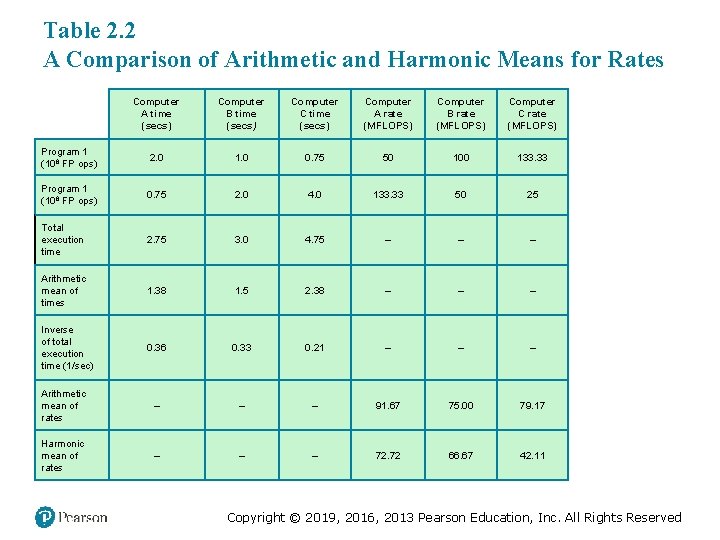
Table 2. 2 A Comparison of Arithmetic and Harmonic Means for Rates Computer A time (secs) Computer B time (secs) Computer C time (secs) Computer A rate (MFLOPS) Computer B rate (MFLOPS) Computer C rate (MFLOPS) Program 1 (108 FP ops) 2. 0 1. 0 0. 75 50 100 133. 33 Program 1 (108 FP ops) 0. 75 2. 0 4. 0 133. 33 50 25 Total execution time 2. 75 3. 0 4. 75 – – – Arithmetic mean of times 1. 38 1. 5 2. 38 – – – Inverse of total execution time (1/sec) 0. 36 0. 33 0. 21 – – – Arithmetic mean of rates – – – 91. 67 75. 00 79. 17 Harmonic mean of rates – – – 72. 72 66. 67 42. 11 Copyright © 2019, 2016, 2013 Pearson Education, Inc. All Rights Reserved

Table 2. 3 A Comparison of Arithmetic and Geometric Means for Normalized Results (a) Results normalized to Computer A time Computer B time Computer C time Program 1 2. 0 (1. 0) 1. 0 (0. 5) 0. 75 (0. 38) Program 2 0. 75 (1. 0) 2. 0 (2. 67) 4. 0 (5. 33) Total execution time 2. 75 3. 0 4. 75 Arithmetic mean of normalized times 1. 00 1. 58 2. 85 Geometric mean of normalized times 1. 00 1. 15 1. 41 (a) Results normalized to Computer B Computer A time Computer B time Computer C time Program 1 2. 0 (2. 0) 1. 0 (1. 0) 0. 75 (0. 75) Program 2 0. 75 (0. 38) 2. 0 (1. 0) 4. 0 (2. 0) Total execution time 2. 75 3. 0 4. 75 Arithmetic mean of normalized times 1. 19 1. 00 1. 38 Geometric mean of normalized times 0. 87 1. 00 1. 22 Copyright © 2019, 2016, 2013 Pearson Education, Inc. All Rights Reserved

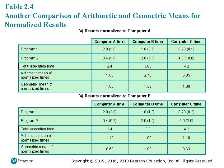
Table 2. 4 Another Comparison of Arithmetic and Geometric Means for Normalized Results (a) Results normalized to Computer A time Computer B time Computer C time Program 1 2. 0 (1. 0) 1. 0 (0. 5) 0. 20 (0. 1) Program 2 0. 4 (1. 0) 2. 0 (5. 0) 4. 0 (10. 0) Total execution time 2. 4 3. 00 4. 2 Arithmetic mean of normalized times 1. 00 2. 75 5. 05 Geometric mean of normalized times 1. 00 1. 58 1. 00 (a) Results normalized to Computer B Computer A time Computer B time Computer C time Program 1 2. 0 (2. 0) 1. 0 (1. 0) 0. 20 (0. 2) Program 2 0. 4 (0. 2) 2. 0 (1. 0) 4. 0 (2. 0) Total execution time 2. 4 3. 0 4. 2 Arithmetic mean of normalized times 1. 10 1. 00 1. 10 Geometric mean of normalized times 0. 63 1. 00 0. 63 Copyright © 2019, 2016, 2013 Pearson Education, Inc. All Rights Reserved

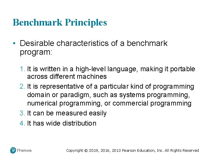
Benchmark Principles • Desirable characteristics of a benchmark program: 1. It is written in a high-level language, making it portable across different machines 2. It is representative of a particular kind of programming domain or paradigm, such as systems programming, numerical programming, or commercial programming 3. It can be measured easily 4. It has wide distribution Copyright © 2019, 2016, 2013 Pearson Education, Inc. All Rights Reserved

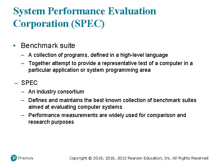
System Performance Evaluation Corporation (SPEC) • Benchmark suite – A collection of programs, defined in a high-level language – Together attempt to provide a representative test of a computer in a particular application or system programming area – SPEC – An industry consortium – Defines and maintains the best known collection of benchmark suites aimed at evaluating computer systems – Performance measurements are widely used for comparison and research purposes Copyright © 2019, 2016, 2013 Pearson Education, Inc. All Rights Reserved

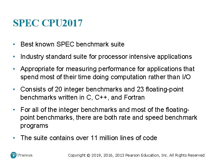
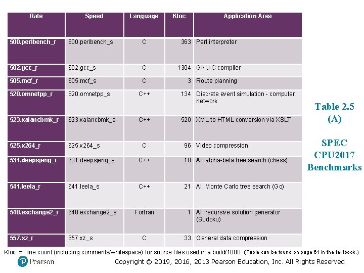
SPEC CPU 2017 • Best known SPEC benchmark suite • Industry standard suite for processor intensive applications • Appropriate for measuring performance for applications that spend most of their time doing computation rather than I/O • Consists of 20 integer benchmarks and 23 floating-point benchmarks written in C, C++, and Fortran • For all of the integer benchmarks and most of the floatingpoint benchmarks, there are both rate and speed benchmark programs • The suite contains over 11 million lines of code Copyright © 2019, 2016, 2013 Pearson Education, Inc. All Rights Reserved

Rate Speed Language Kloc Application Area 500. perlbench_r 600. perlbench_s C 363 Perl interpreter 502. gcc_r 602. gcc_s C 1304 GNU C compiler 505. mcf_r 605. mcf_s C 520. omnetpp_r 620. omnetpp_s C++ 3 Route planning 134 Discrete event simulation - computer network 523. xalancbmk_r 623. xalancbmk_s 525. x 264_r 625. x 264_s 531. deepsjeng_r 631. deepsjeng_s C++ 10 AI: alpha-beta tree search (chess) 541. leela_r 641. leela_s C++ 21 AI: Monte Carlo tree search (Go) 548. exchange 2_r 648. exchange 2_s Fortran 1 AI: recursive solution generator (Sudoku) 557. xz_r 657. xz_s C C 520 XML to HTML conversion via XSLT 96 Video compression Table 2. 5 (A) SPEC CPU 2017 Benchmarks 33 General data compression Kloc = line count (including comments/whitespace) for source files used in a build/1000 (Table can be found on page 61 in the textbook. ) Copyright © 2019, 2016, 2013 Pearson Education, Inc. All Rights Reserved

Rate Speed Language 503. bwaves_r 603. bwaves_s Fortran 507. cactu. BSSN_r 607. cactu. BSSN_s C++, C, Fortran Kloc Application Area 1 Explosion modeling 257 Physics; relativity 508. namd_r C++, C 510. parest_r C++ 427 Biomedical imaging; optical tomography with finite elements 511. povray_r C++ 170 Ray tracing 519. ibm_r 619. ibm_s C 521. wrf_r 621. wrf_s Fortran, C 526. blender_r 527. cam 4_r C++ 8 Molecular dynamics 1 Fluid dynamics 991 Weather forecasting 1577 3 D rendering and animation 627. cam 4_s Fortran, C 407 Atmosphere modeling 628. pop 2_s Fortran, C 338 Wide-scale ocean modeling (climate level) 538. imagick_r 638. imagick_s C 259 Image manipulation 544. nab_r 644. nab_s C 24 Molecular dynamics 549. fotonik 3 d_r 649. fotonik 3 d_s Fortran 554. roms_r 654. roms_s Fortran Table 2. 5 (B) SPEC CPU 2017 Benchmarks 14 Computational electromagnetics 210 Regional ocean modeling. Kloc = line count (including comments/whitespace) for source files used in a build/1000 (Table can be found on page 61 in the textbook. ) Copyright © 2019, 2016, 2013 Pearson Education, Inc. All Rights Reserved

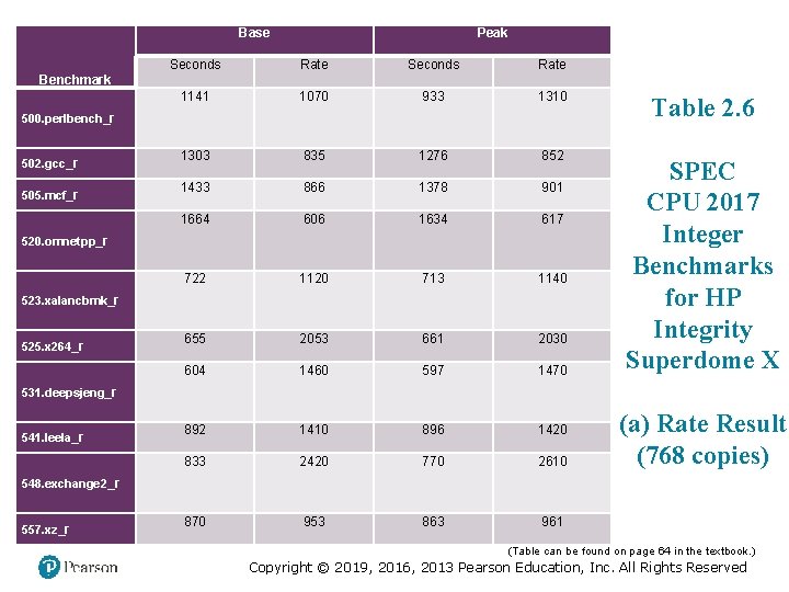
Base Peak Seconds Rate 1141 1070 933 1310 1303 835 1276 852 1433 866 1378 901 1664 606 1634 617 722 1120 713 1140 655 2053 661 2030 604 1460 597 1470 892 1410 896 1420 833 2420 770 2610 870 953 863 961 Benchmark 500. perlbench_r 502. gcc_r 505. mcf_r 520. omnetpp_r 523. xalancbmk_r 525. x 264_r Table 2. 6 SPEC CPU 2017 Integer Benchmarks for HP Integrity Superdome X 531. deepsjeng_r 541. leela_r (a) Rate Result (768 copies) 548. exchange 2_r 557. xz_r © 2018 Pearson Education, Inc. , Hoboken, NJ. All rights reserved. (Table can be found on page 64 in the textbook. ) Copyright © 2019, 2016, 2013 Pearson Education, Inc. All Rights Reserved

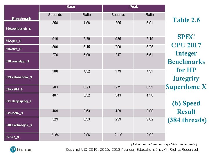
Base Peak Seconds Ratio 358 4. 96 295 6. 01 546 7. 29 535 7. 45 866 5. 45 700 6. 75 276 5. 90 247 6. 61 188 7. 52 179 7. 91 283 6. 23 271 6. 51 407 3. 52 343 4. 18 Benchmark Table 2. 6 600. perlbench_s 602. gcc_s 605. mcf_s 620. omnetpp_s 623. xalancbmk_s 625. x 264_s 631. deepsjeng_s 641. leela_s 469 3. 63 439 3. 88 329 8. 93 299 9. 82 2164 2. 86 2119 2. 92 648. exchange 2_s 657. xz_s SPEC CPU 2017 Integer Benchmarks for HP Integrity Superdome X (b) Speed Result (384 threads) (Table can be found on page 64 in the textbook. ) Copyright © 2019, 2016, 2013 Pearson Education, Inc. All Rights Reserved

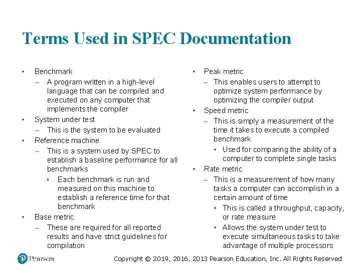
Terms Used in SPEC Documentation • • Benchmark – A program written in a high-level language that can be compiled and executed on any computer that implements the compiler System under test – This is the system to be evaluated Reference machine – This is a system used by SPEC to establish a baseline performance for all benchmarks ▪ Each benchmark is run and measured on this machine to establish a reference time for that benchmark Base metric – These are required for all reported results and have strict guidelines for compilation • • • Peak metric – This enables users to attempt to optimize system performance by optimizing the compiler output Speed metric – This is simply a measurement of the time it takes to execute a compiled benchmark • Used for comparing the ability of a computer to complete single tasks Rate metric – This is a measurement of how many tasks a computer can accomplish in a certain amount of time • This is called a throughput, capacity, or rate measure • Allows the system under test to execute simultaneous tasks to take advantage of multiple processors Copyright © 2019, 2016, 2013 Pearson Education, Inc. All Rights Reserved

Figure 2. 7 Copyright © 2019, 2016, 2013 Pearson Education, Inc. All Rights Reserved

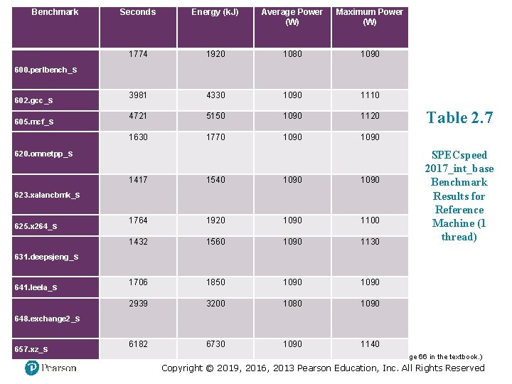
Benchmark Seconds Energy (k. J) Average Power (W) Maximum Power (W) 1774 1920 1080 1090 3981 4330 1090 1110 4721 5150 1090 1120 1630 1770 1090 600. perlbench_s 602. gcc_s 605. mcf_s 620. omnetpp_s 1417 1540 1090 1764 1920 1090 1100 1432 1560 1090 1130 1706 1850 1090 2939 3200 1080 1090 6182 6730 1090 1140 623. xalancbmk_s 625. x 264_s Table 2. 7 SPECspeed 2017_int_base Benchmark Results for Reference Machine (1 thread) 631. deepsjeng_s 641. leela_s 648. exchange 2_s 657. xz_s (Table can be found on page 66 in the textbook. ) Copyright © 2019, 2016, 2013 Pearson Education, Inc. All Rights Reserved

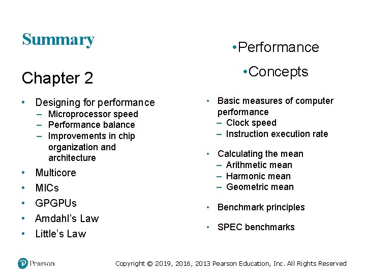
Summary • Performance • Concepts Chapter 2 • Designing for performance – Microprocessor speed – Performance balance – Improvements in chip organization and architecture • • • Multicore MICs GPGPUs Amdahl’s Law Little’s Law • Basic measures of computer performance – Clock speed – Instruction execution rate • Calculating the mean – Arithmetic mean – Harmonic mean – Geometric mean • Benchmark principles • SPEC benchmarks Copyright © 2019, 2016, 2013 Pearson Education, Inc. All Rights Reserved

Copyright This work is protected by United States copyright laws and is provided solely for the use of instructions in teaching their courses and assessing student learning. dissemination or sale of any part of this work (including on the World Wide Web) will destroy the integrity of the work and is not permitted. The work and materials from it should never be made available to students except by instructors using the accompanying text in their classes. All recipients of this work are expected to abide by these restrictions and to honor the intended pedagogical purposes and the needs of other instructors who rely on these materials. Copyright © 2019, 2016, 2013 Pearson Education, Inc. All Rights Reserved