Computer Graphics Week 10 Lecture 1 Splines Modelling

Computer Graphics Week 10 Lecture 1

Splines (Modelling Curves)

Question Before the advent of sophisticated Computers how did people draw curves accurately ?

Spline : Flexible strip used to draw curves through designated points

Splines • Originally , the curves drawn with spline were called Spline curves. • Splines are now used to model a variety of curves (natural and artificial) • We usually mathematically model them using piecewise cubic functions (1 st and 2 nd derivatives are continuous) spline curve now refers to any composite curve formed with polynomial sections satisfying any specified continuity conditions at the boundary of the pieces

Uses of Splines Use of approximate naturally occurring curves (landscape, leaves, astronomical bodies , electron orbitals) Design curves Digitize drawings Specify animation paths CAD uses splines for design of automobile bodies , surfaces of aircraft and space crafts, ship hulls and home appliances

We specify Splines by a set of coordinate points called Control Points , which indicate the general shape of the curve. Based on how control points are used , there are 2 drawing techniques: 1. Interpolation 2. Approximation

Interpolation and Approximation Interpolation Approximation When polynomial sections are fitted such that all control points are connected When a polynomial curve is fitted such that some or all the control points are not on the generated curve The control points specify the general path of the curve

Parametric continuity Constraints To ensure smooth transition from one section of spline to the next we impose various continuity constraints A cubic curve section can be parameterized as follow:

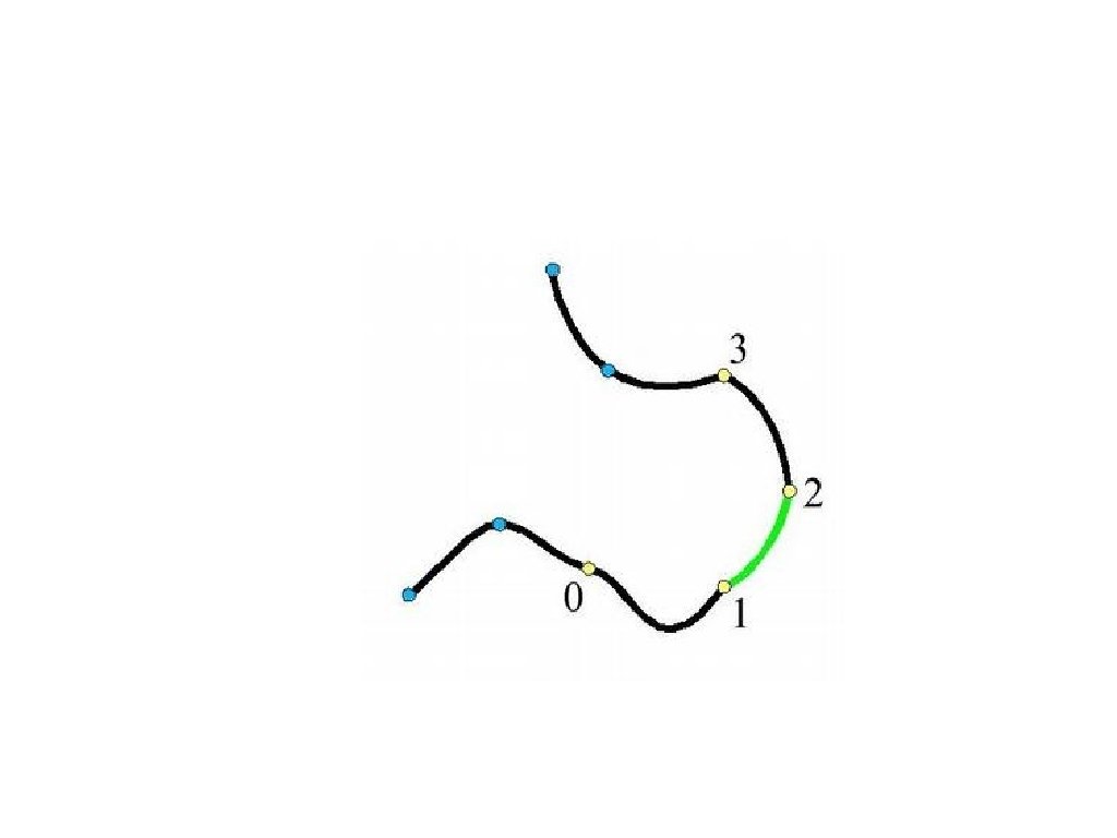
Zero Order Parametric Continuity represented as C 0 , it simply means that the two curves meet at a common point. The endpoint of first curve is the starting point of the successive curve First Order Parametric Continuity represented as C 1 , Here Additionally , the first parametric derivative (tangent) of the two curves is same at the meeting point Second Order Parametric Continuity represented as C 2 , Here Additionally , the second parametric derivative of the two curves is same at the meeting point as well i. e. the rate of change of tangent of the 2 curves is also same

There are 3 equivalent methods for specifying a Spline spline: 1. Stating set of boundary conditions on the spline Specific 2. Stating a matrix that specifies a spline ation 3. Stating set of blending functions (or basis functions) that determine how specified constraints are combined to calculate curve

Cubic interpolation methods • In these methods the piecewise curves are cubic polynomials • Benefits of cubic polynomials → Speed and flexibility • Given n+1 control points : Our need is to fit cubic curves between adjacent control points. For each curve we can define coordinates that lie on the curve in cubic parametric eq:

Contd. . . - We can find equation of each curve by finding the values of coefficients a, b, c, d for each piecewise curve We impose continuity contraints to find these coefficients

Interpolation Methods We will look at 2 interpolation methods: - Natural Cubic Interpolation (the simplest one) - Hermite Interpolation

Natural Cubic Interpolation - Simplest method Suppose we have n+1 control points ⇒ We need to draw n curves For each curve we need to know 4 coefficients (a, b, c, d) → Need 4 equations (or 4 boundary conditions) Conditions on board No “local” control

Hermite Method - Developed by French Mathematician, Charles Hermite Allow for more local control Require specified tangent at each control point

Hermite Method Here P(u) → eq. of curve section , pk → control point k Then in Hermite method the boundary conditions that define the curve are:

Hermite Method(matrix form) The curve equation : can be expressed in vector form as : which can be written in matrix form as (eq. 1):

contd. . . Taking derivative wrt u: Now since we know P(u) and P’(u) we can rewrite our boundary conditions as:

contd. . . Putting coefficients value back in eq 1 :

Hermite Method (blending func. form) - Multiplying the previous matrix equation we get: Here H 0, H 1, H 2, H 3 are Hermite blending functions.

contd. . .

Hermite Method ➔Issue with Hermite function ➔Variation : ◆Cardinal splines ◆Kochanek-Bartels

The End

Splines Originally , the curves drawn with spline were called Spline curves. Splines are now used to model a variety of curves (natural and artificial) We mathematically model them using

Text

Text

Text –Johnny Appleseed