Computer Graphics Lecture 3 Transformations 30102020 Lecture 4

Computer Graphics Lecture 3 Transformations 30/10/2020 Lecture 4 1

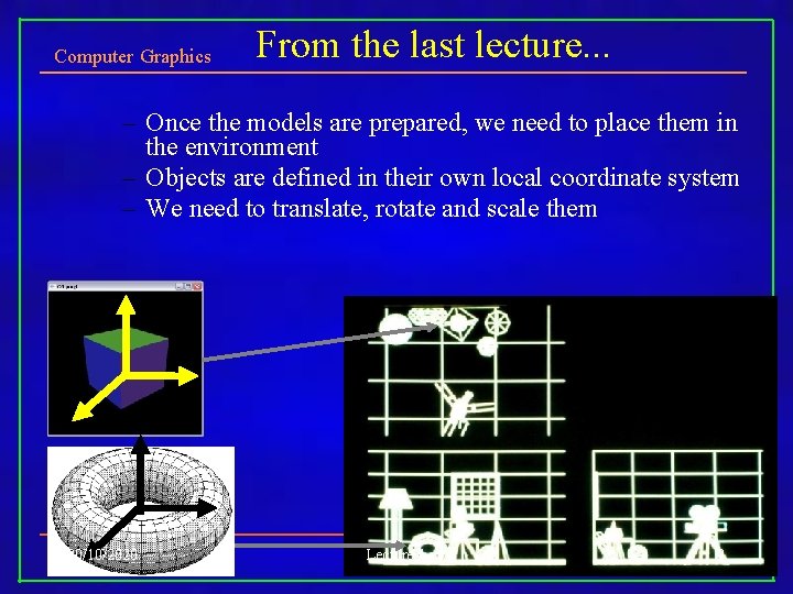
Computer Graphics From the last lecture. . . – Once the models are prepared, we need to place them in the environment – Objects are defined in their own local coordinate system – We need to translate, rotate and scale them 30/10/2020 Lecture 4 2

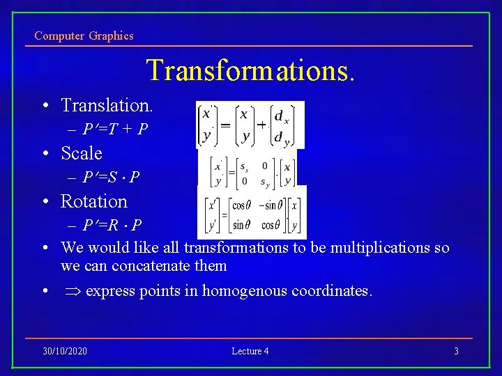
Computer Graphics Transformations. • Translation. – P =T + P • Scale – P =S P • Rotation – P =R P • We would like all transformations to be multiplications so we can concatenate them • express points in homogenous coordinates. 30/10/2020 Lecture 4 3

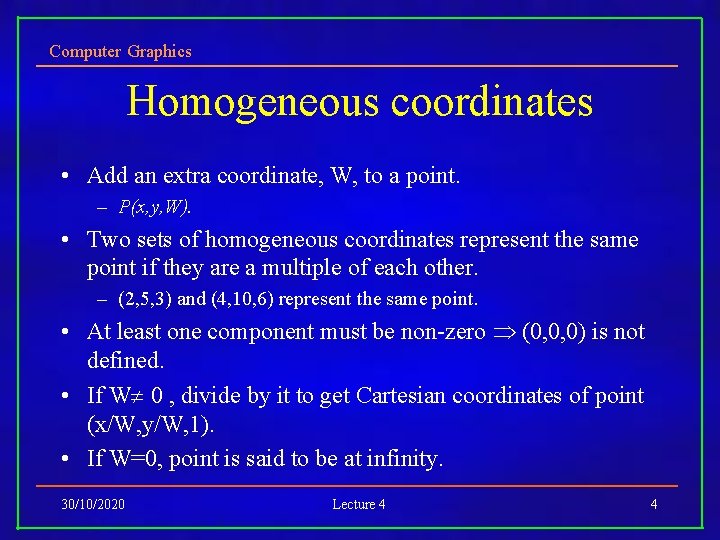
Computer Graphics Homogeneous coordinates • Add an extra coordinate, W, to a point. – P(x, y, W). • Two sets of homogeneous coordinates represent the same point if they are a multiple of each other. – (2, 5, 3) and (4, 10, 6) represent the same point. • At least one component must be non-zero (0, 0, 0) is not defined. • If W 0 , divide by it to get Cartesian coordinates of point (x/W, y/W, 1). • If W=0, point is said to be at infinity. 30/10/2020 Lecture 4 4

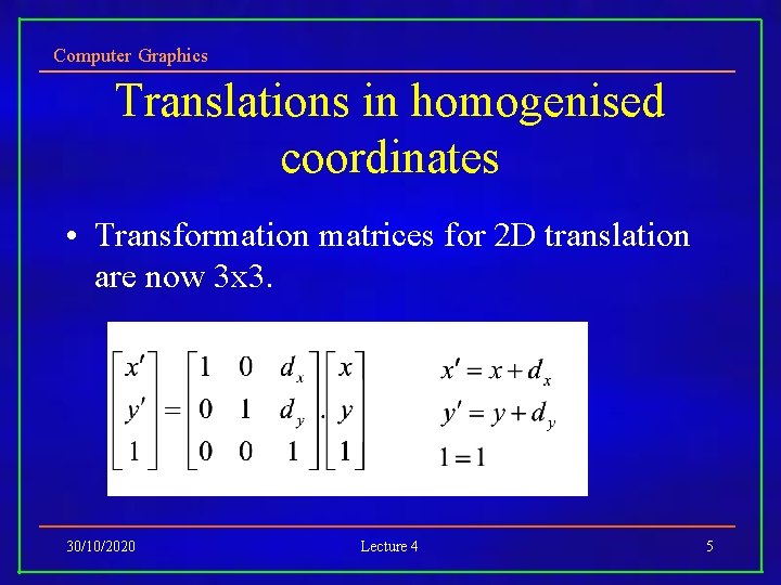
Computer Graphics Translations in homogenised coordinates • Transformation matrices for 2 D translation are now 3 x 3. 30/10/2020 Lecture 4 5

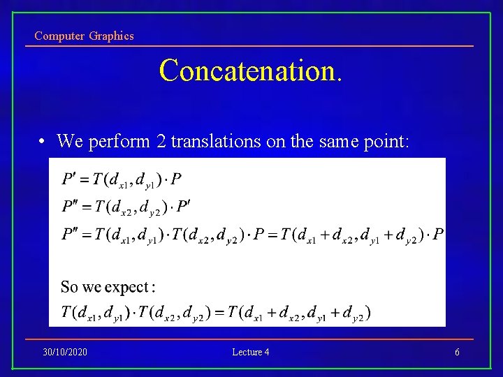
Computer Graphics Concatenation. • We perform 2 translations on the same point: 30/10/2020 Lecture 4 6

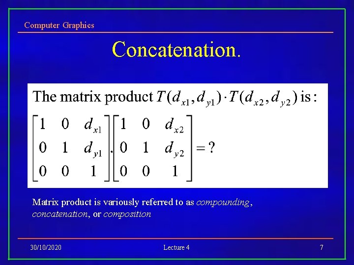
Computer Graphics Concatenation. Matrix product is variously referred to as compounding, concatenation, or composition 30/10/2020 Lecture 4 7

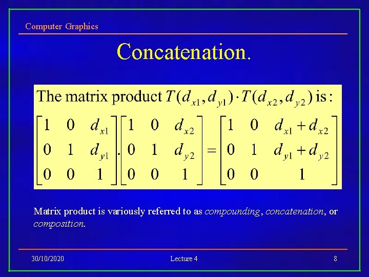
Computer Graphics Concatenation. Matrix product is variously referred to as compounding, concatenation, or composition. 30/10/2020 Lecture 4 8

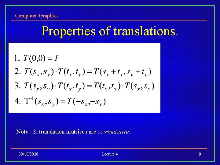
Computer Graphics Properties of translations. Note : 3. translation matrices are commutative. 30/10/2020 Lecture 4 9

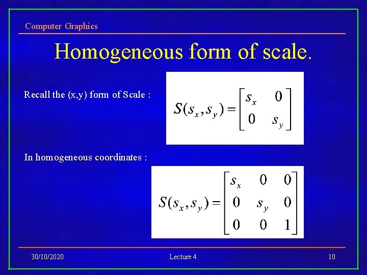
Computer Graphics Homogeneous form of scale. Recall the (x, y) form of Scale : In homogeneous coordinates : 30/10/2020 Lecture 4 10

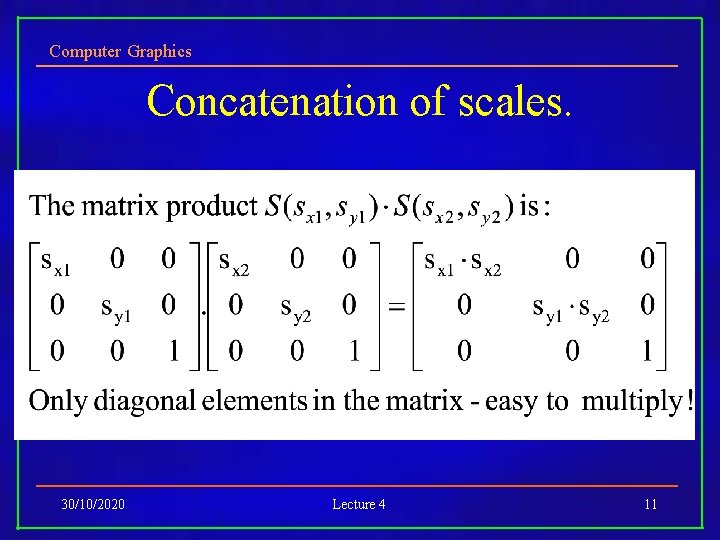
Computer Graphics Concatenation of scales. 30/10/2020 Lecture 4 11

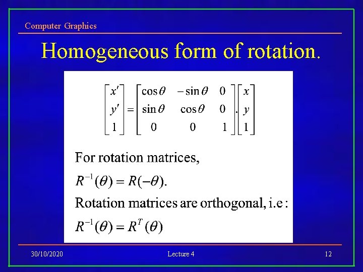
Computer Graphics Homogeneous form of rotation. 30/10/2020 Lecture 4 12

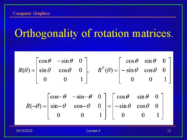
Computer Graphics Orthogonality of rotation matrices. 30/10/2020 Lecture 4 13

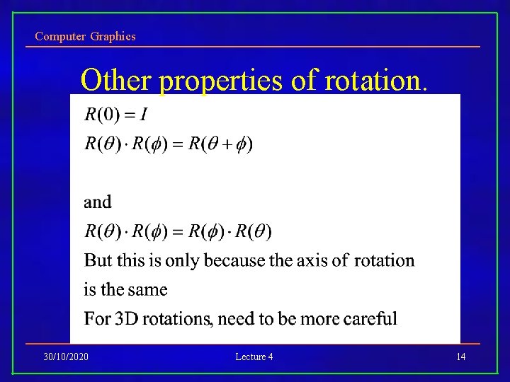
Computer Graphics Other properties of rotation. 30/10/2020 Lecture 4 14

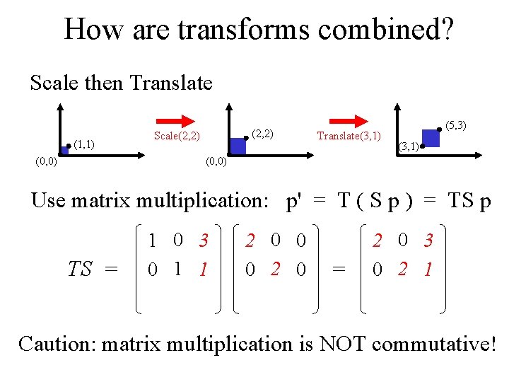
How are transforms combined? Computer Graphics Scale then Translate (1, 1) (2, 2) Scale(2, 2) Translate(3, 1) (5, 3) (3, 1) (0, 0) Use matrix multiplication: p' = T ( S p ) = TS p TS = 1 0 3 0 1 1 2 0 0 0 2 0 = 2 0 3 0 2 1 Caution: matrix multiplication is NOT commutative! 30/10/2020 Lecture 4 15

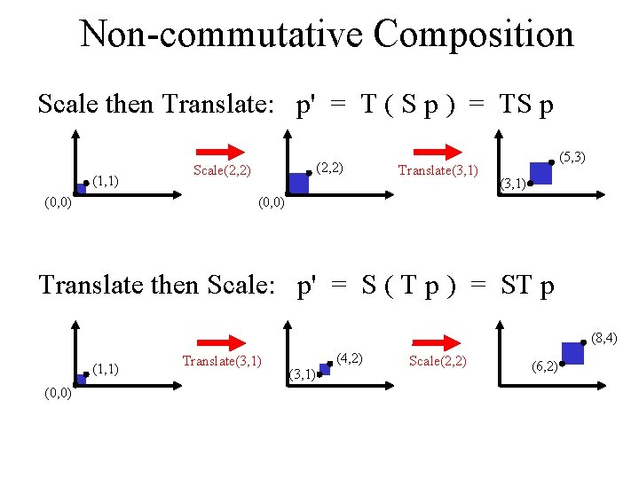
Non-commutative Composition Computer Graphics Scale then Translate: p' = T ( S p ) = TS p (1, 1) (2, 2) Scale(2, 2) Translate(3, 1) (5, 3) (3, 1) (0, 0) Translate then Scale: p' = S ( T p ) = ST p (8, 4) (1, 1) Translate(3, 1) (4, 2) (3, 1) Scale(2, 2) (6, 2) (0, 0) 30/10/2020 Lecture 4 16

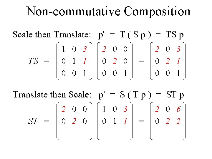
Non-commutative Composition Computer Graphics Scale then Translate: p' = T ( S p ) = TS p TS = 1 0 3 0 1 1 0 0 1 2 0 0 0 1 = 2 0 3 0 2 1 0 0 1 Translate then Scale: p' = S ( T p ) = ST p ST = 30/10/2020 2 0 0 0 2 0 1 0 3 0 1 1 Lecture 4 = 2 0 6 0 2 2 17

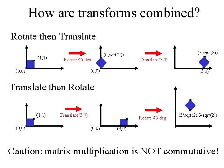
How are transforms combined? Computer Graphics Rotate then Translate (1, 1) Rotate 45 deg (0, sqrt(2)) (3, sqrt(2)) Translate(3, 0) (0, 0) (3, 0) Translate then Rotate (1, 1) (0, 0) Translate(3, 0) Rotate 45 deg (0, 0) (3/sqrt(2), 3/sqrt(2)) (3, 0) Caution: matrix multiplication is NOT commutative! 30/10/2020 Lecture 4 18

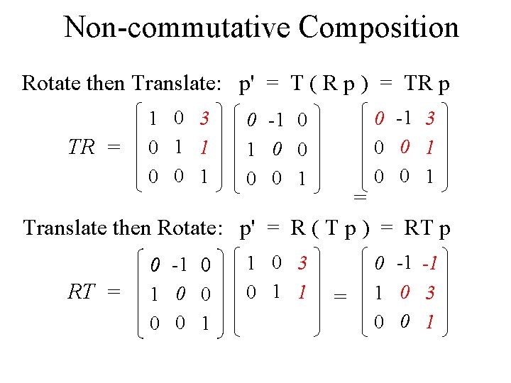
Non-commutative Composition Computer Graphics Rotate then Translate: p' = T ( R p ) = TR p TR = 1 0 3 0 1 1 0 0 1 0 -1 0 0 0 0 1 0 -1 3 0 0 1 0 -1 0 0 0 0 1 1 0 3 0 1 1 0 -1 -1 1 0 3 0 0 1 = Translate then Rotate: p' = R ( T p ) = RT p RT = 30/10/2020 Lecture 4 = 19

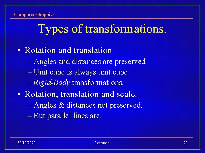
Computer Graphics Types of transformations. • Rotation and translation – Angles and distances are preserved – Unit cube is always unit cube – Rigid-Body transformations. • Rotation, translation and scale. – Angles & distances not preserved. – But parallel lines are. 30/10/2020 Lecture 4 20

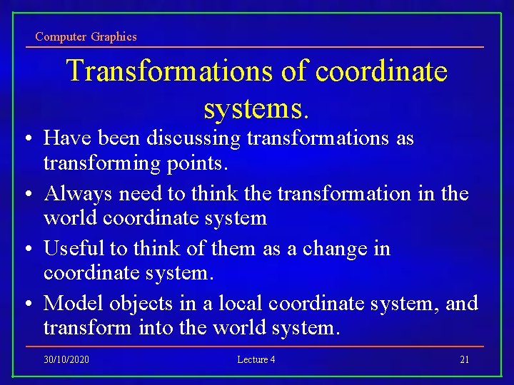
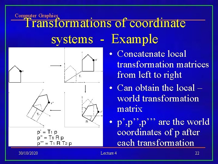
Computer Graphics Transformations of coordinate systems. • Have been discussing transformations as transforming points. • Always need to think the transformation in the world coordinate system • Useful to think of them as a change in coordinate system. • Model objects in a local coordinate system, and transform into the world system. 30/10/2020 Lecture 4 21

Computer Graphics Transformations of coordinate systems - Example • Concatenate local transformation matrices from left to right • Can obtain the local – world transformation matrix • p’, p’’’ are the world coordinates of p after each transformation 30/10/2020 Lecture 4 22

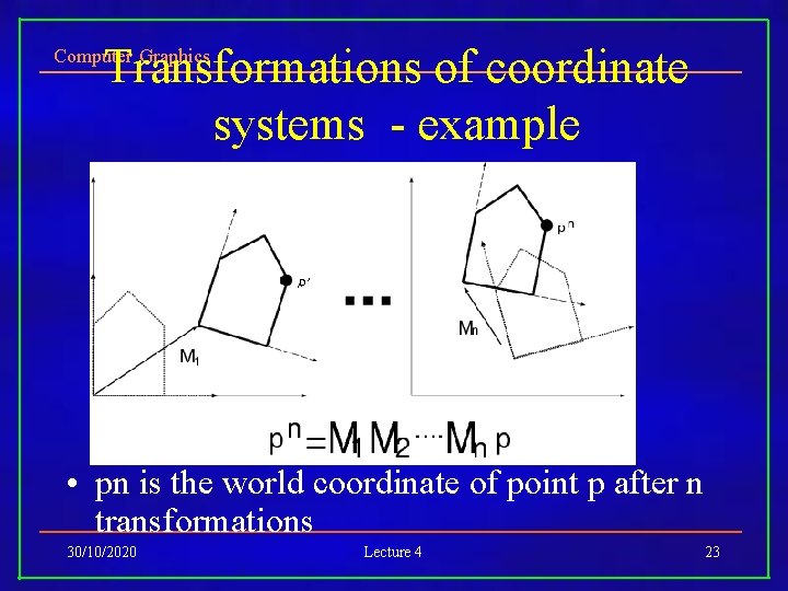
Transformations of coordinate systems - example Computer Graphics • pn is the world coordinate of point p after n transformations 30/10/2020 Lecture 4 23

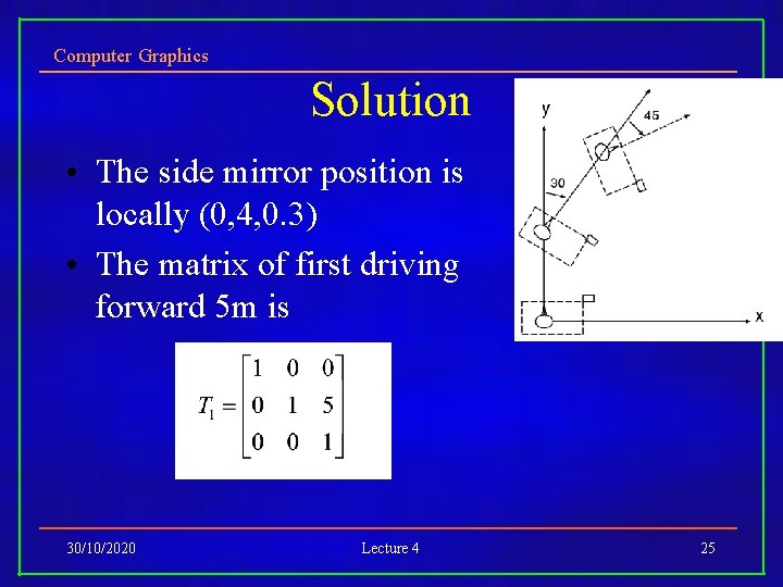
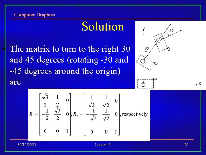
Computer Graphics Quiz • I sat in the car, and realized the side mirror is 0. 4 m on my right and 0. 3 m in my front • I started my car and drove 5 m forward, turned 30 degrees to right, moved 5 m forward again, and turned 45 degrees to the right, and stopped • What is the position of the side mirror now, relative to where I was sitting in the beginning? 30/10/2020 Lecture 4 24

Computer Graphics Solution • The side mirror position is locally (0, 4, 0. 3) • The matrix of first driving forward 5 m is 30/10/2020 Lecture 4 25

Computer Graphics Solution • The matrix to turn to the right 30 and 45 degrees (rotating -30 and -45 degrees around the origin) are 30/10/2020 Lecture 4 26

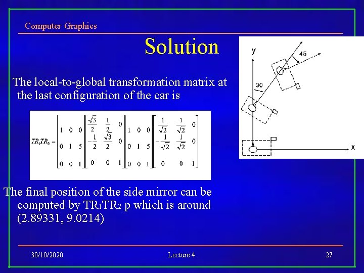
Computer Graphics Solution The local-to-global transformation matrix at the last configuration of the car is The final position of the side mirror can be computed by TR 1 TR 2 p which is around (2. 89331, 9. 0214) 30/10/2020 Lecture 4 27

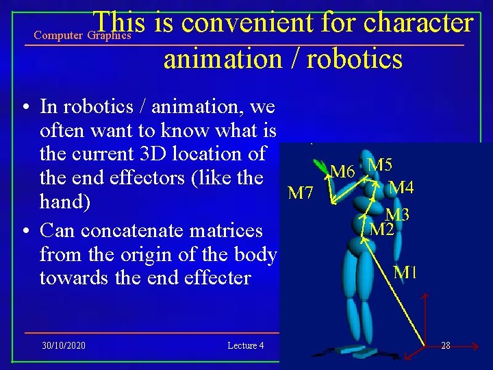
This is convenient for character animation / robotics Computer Graphics • In robotics / animation, we often want to know what is the current 3 D location of the end effectors (like the hand) • Can concatenate matrices from the origin of the body towards the end effecter 30/10/2020 Lecture 4 28

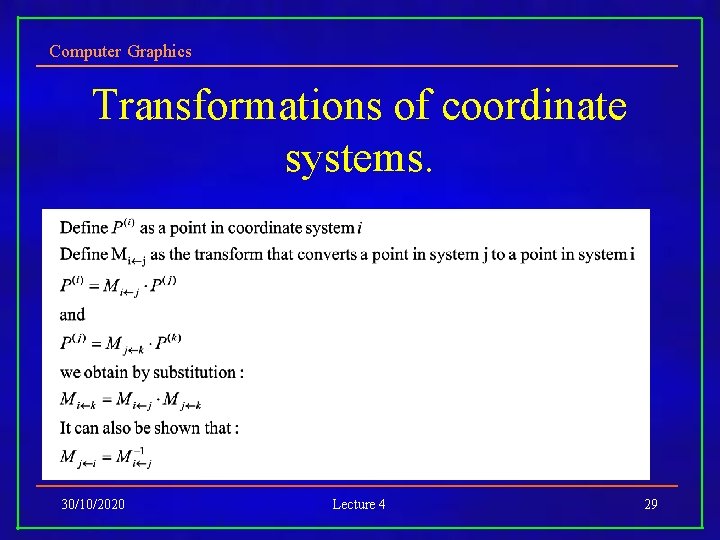
Computer Graphics Transformations of coordinate systems. 30/10/2020 Lecture 4 29

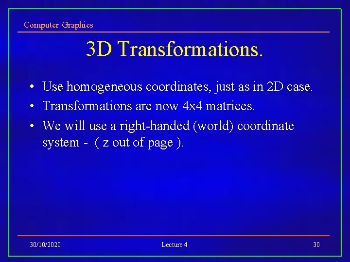
Computer Graphics 3 D Transformations. • Use homogeneous coordinates, just as in 2 D case. • Transformations are now 4 x 4 matrices. • We will use a right-handed (world) coordinate system - ( z out of page ). 30/10/2020 Lecture 4 30

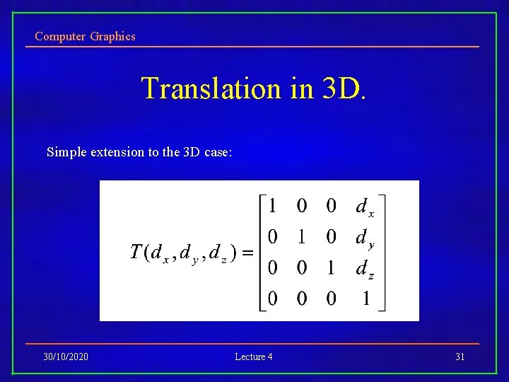
Computer Graphics Translation in 3 D. Simple extension to the 3 D case: 30/10/2020 Lecture 4 31

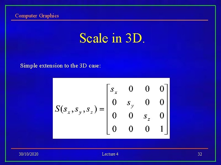
Computer Graphics Scale in 3 D. Simple extension to the 3 D case: 30/10/2020 Lecture 4 32

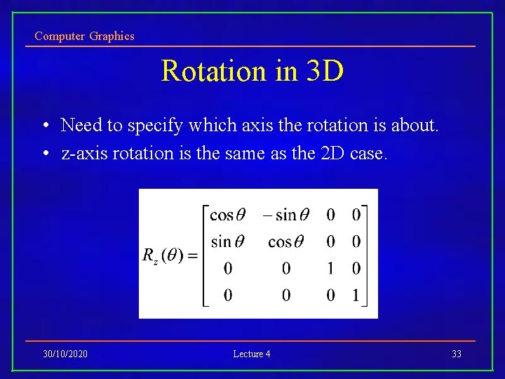
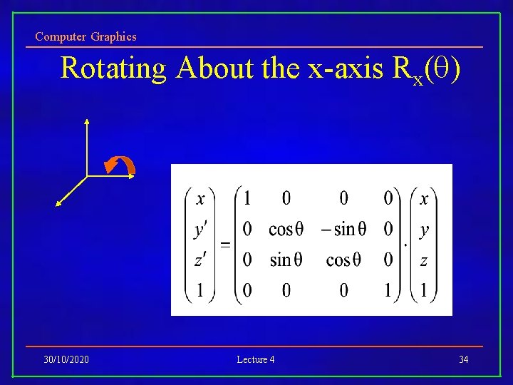
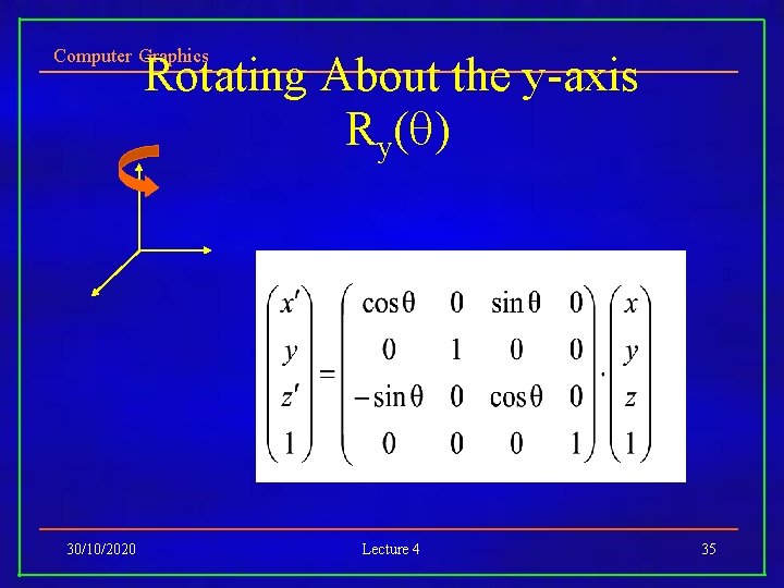
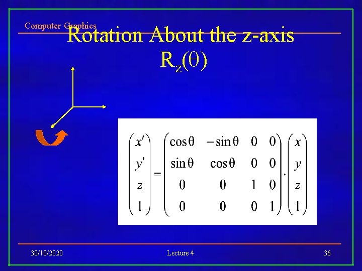
Computer Graphics Rotation in 3 D • Need to specify which axis the rotation is about. • z-axis rotation is the same as the 2 D case. 30/10/2020 Lecture 4 33

Computer Graphics Rotating About the x-axis Rx( ) 30/10/2020 Lecture 4 34

Computer Graphics Rotating About the y-axis Ry( ) 30/10/2020 Lecture 4 35

Computer Graphics Rotation About the z-axis Rz( ) 30/10/2020 Lecture 4 36

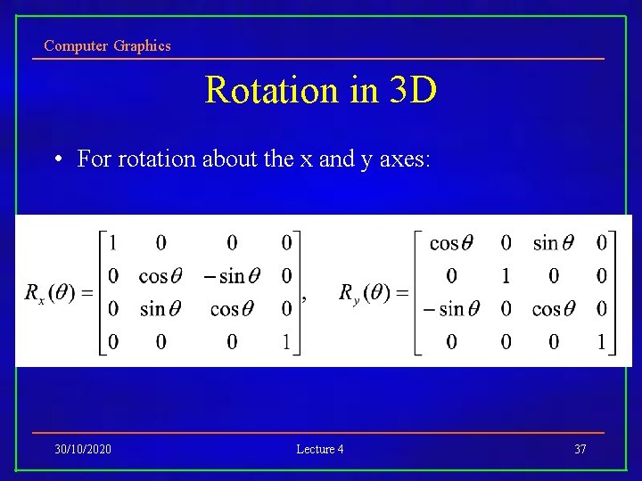
Computer Graphics Rotation in 3 D • For rotation about the x and y axes: 30/10/2020 Lecture 4 37

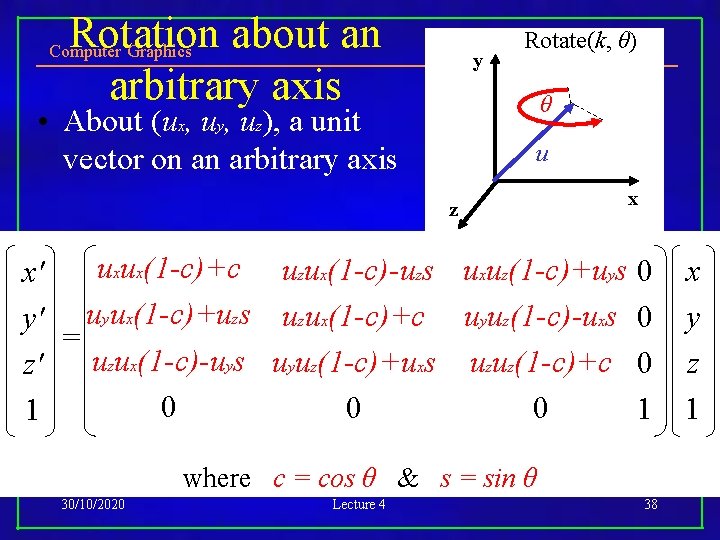
Rotation about an arbitrary axis Computer Graphics y Rotate(k, θ) θ • About (ux, uy, uz), a unit vector on an arbitrary axis u z x uxux(1 -c)+c uzux(1 -c)-uzs uxuz(1 -c)+uys 0 x' y' uyux(1 -c)+uzs uzux(1 -c)+c uyuz(1 -c)-uxs 0 = uzux(1 -c)-uys uyuz(1 -c)+uxs uzuz(1 -c)+c 0 z' 0 0 0 1 1 where c = cos θ & s = sin θ 30/10/2020 Lecture 4 38 x y z 1

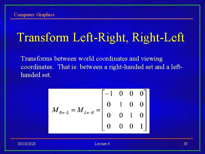
Computer Graphics Transform Left-Right, Right-Left Transforms between world coordinates and viewing coordinates. That is: between a right-handed set and a lefthanded set. 30/10/2020 Lecture 4 39

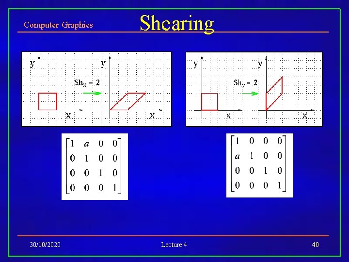
Computer Graphics 30/10/2020 Shearing Lecture 4 40

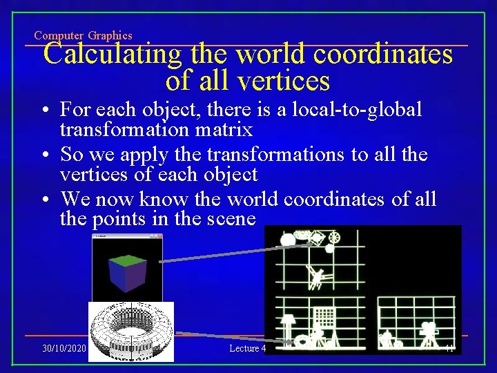
Computer Graphics Calculating the world coordinates of all vertices • For each object, there is a local-to-global transformation matrix • So we apply the transformations to all the vertices of each object • We now know the world coordinates of all the points in the scene 30/10/2020 Lecture 4 41

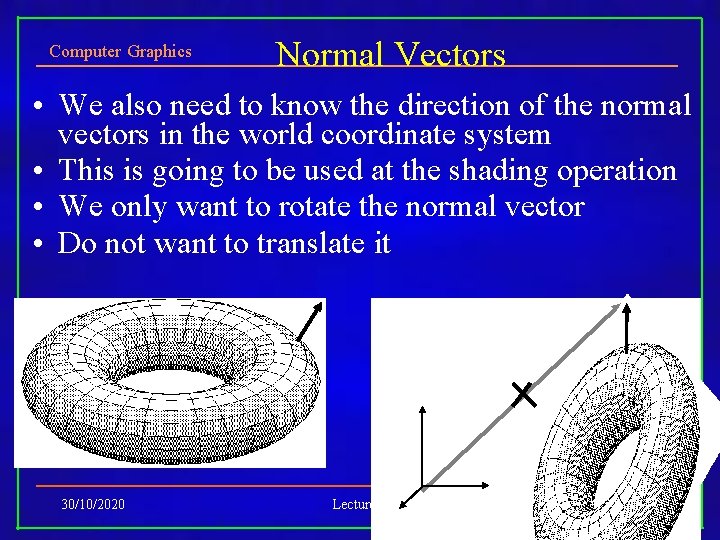
Computer Graphics Normal Vectors • We also need to know the direction of the normal vectors in the world coordinate system • This is going to be used at the shading operation • We only want to rotate the normal vector • Do not want to translate it 30/10/2020 Lecture 4 42

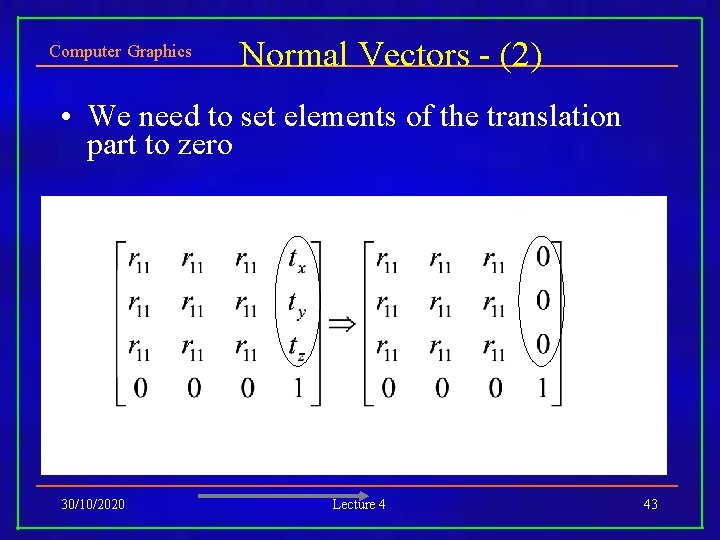
Computer Graphics Normal Vectors - (2) • We need to set elements of the translation part to zero 30/10/2020 Lecture 4 43

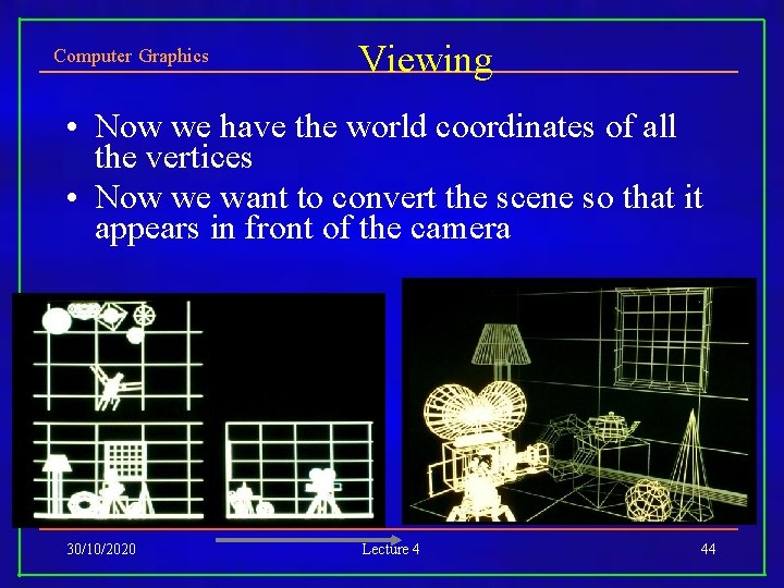
Computer Graphics Viewing • Now we have the world coordinates of all the vertices • Now we want to convert the scene so that it appears in front of the camera 30/10/2020 Lecture 4 44

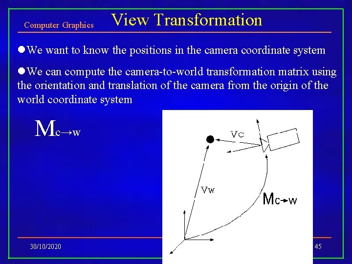
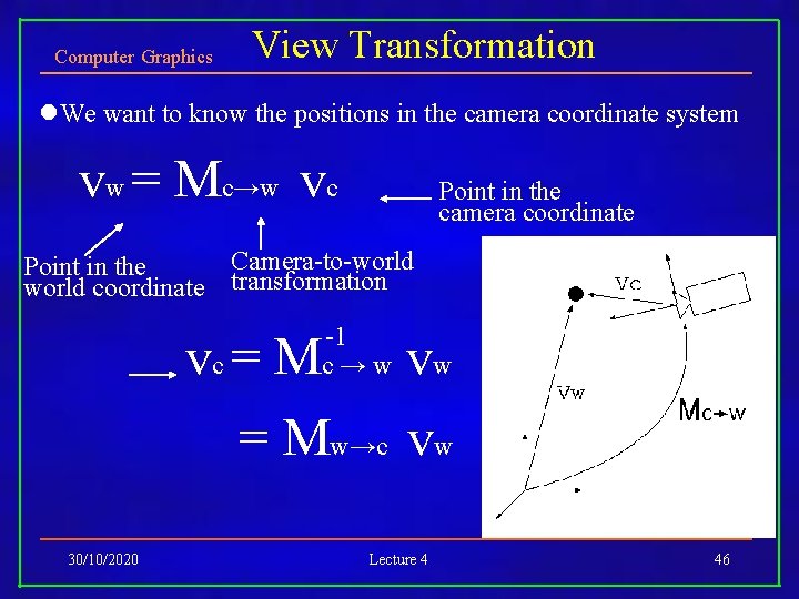
Computer Graphics View Transformation We want to know the positions in the camera coordinate system We can compute the camera-to-world transformation matrix using the orientation and translation of the camera from the origin of the world coordinate system Mc→w 30/10/2020 Lecture 4 45

Computer Graphics View Transformation We want to know the positions in the camera coordinate system vw = Mc→w vc Point in the camera coordinate Camera-to-world Point in the world coordinate transformation vc = M -1 c→w vw = Mw→c vw 30/10/2020 Lecture 4 46

Computer Graphics Summary. • Using homogeneous transformation, translation, rotation and scaling can all be represented by multiplication of a 4 x 4 matrix • Multiplication from left-to-right can be considered as the transformation of the coordinate system • Need to multiply the camera matrix from the left at the end • Reading: Foley et al. Chapter 5, Appendix 2 sections A 1 to A 5 for revision and further background (Chapter 5) 30/10/2020 Lecture 4 47