Computer graphics III Multiple Importance Sampling Jaroslav Kivnek

Computer graphics III – Multiple Importance Sampling Jaroslav Křivánek, MFF UK Jaroslav. Krivanek@mff. cuni. cz

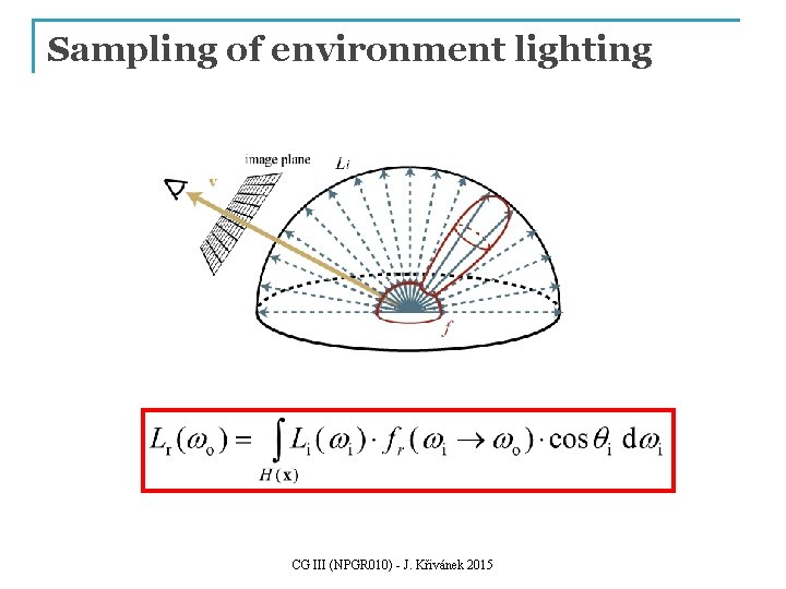
Sampling of environment lighting CG III (NPGR 010) - J. Křivánek 2015

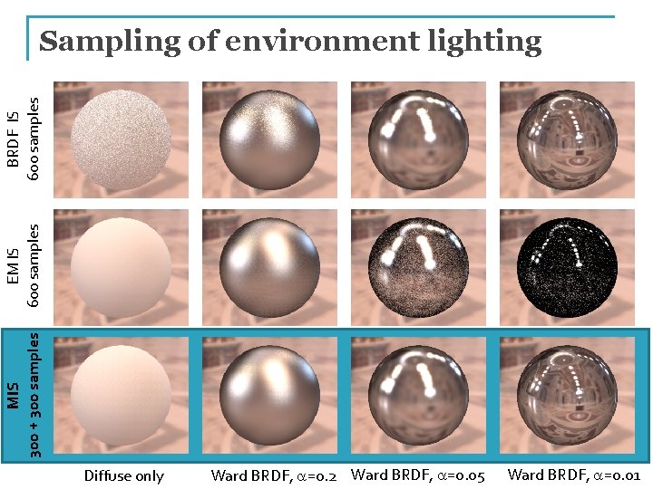
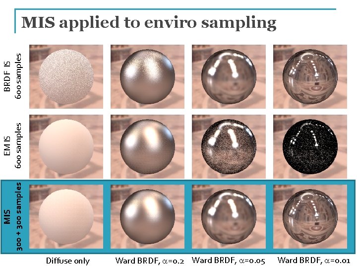
MIS 300 + 300 samples EM IS 600 samples BRDF IS 600 samples Sampling of environment lighting Diffuse only Ward BRDF, a=0. 2 Ward BRDF, a=0. 05 Ward BRDF, a=0. 01

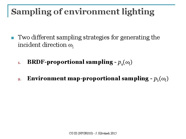
Sampling of environment lighting n Two different sampling strategies for generating the incident direction wi 1. BRDF-proportional sampling - pa(wi) 2. Environment map-proportional sampling - pb(wi) CG III (NPGR 010) - J. Křivánek 2015

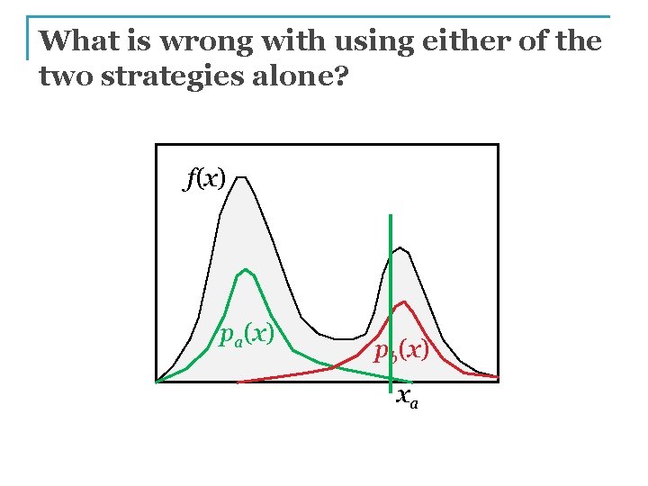
What is wrong with using either of the two strategies alone? f(x) pa(x) pb(x) xa

Notes on the previous slide n n n n n We have a complex multimodal integrand f(x) that we want to numerically integrate using a MC method with importance sampling. Unfortunately, we do not have a PDF that would mimic the integrand in the entire domain. Instead, we can draw the sample from two different PDFs, pa and pb each of which is a good match for the integrand under different conditions – i. e. in different part of the domain. However, the estimators corresponding to these two PDFs have extremely high variance – shown on the slide. We can use Multiple Importance Sampling (MIS) to combine the sampling techniques corresponding to the two PDFs into a single, robust, combined technique. The MIS procedure is extremely simple: sample from both techniques pa and pb , and then takes the sample from the selected distribution. This estimator is really powerful at suppressing outlier samples such as those that you would obtain by picking x_from the tail of pa, where f(x) might still be large. Without having pb at our disposal, we would be dividing the large f(x) by the small pa (x), producing an outlier. However, the combined technique has a much higher chance of producing this particular x (because it can sample it also from pb), so the combined estimator divides f(x) by [pa (x) + pb(x)] / 2, which yields a much more reasonable sample value. I want to note that what I’m showing here is called the “balance heuristic” and is a part of a wider theory on weighted combinations of estimators proposed by Veach and Guibas. CG III (NPGR 010) - J. Křivánek 2015

Multiple Importance Sampling First for general estimators, so please forget the direct illumination problem for a short while.

n. Start with enviro example CG III (NPGR 010) - J. Křivánek 2015

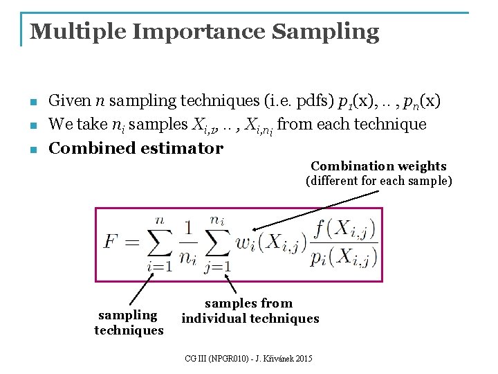
Multiple Importance Sampling n n n Given n sampling techniques (i. e. pdfs) p 1(x), . . , pn(x) We take ni samples Xi, 1, . . , Xi, ni from each technique Combined estimator Combination weights (different for each sample) sampling techniques samples from individual techniques CG III (NPGR 010) - J. Křivánek 2015

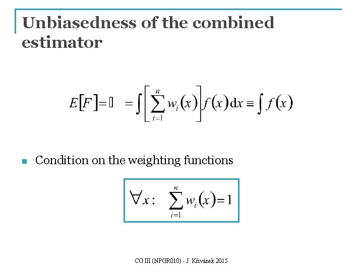
Unbiasedness of the combined estimator n Condition on the weighting functions CG III (NPGR 010) - J. Křivánek 2015

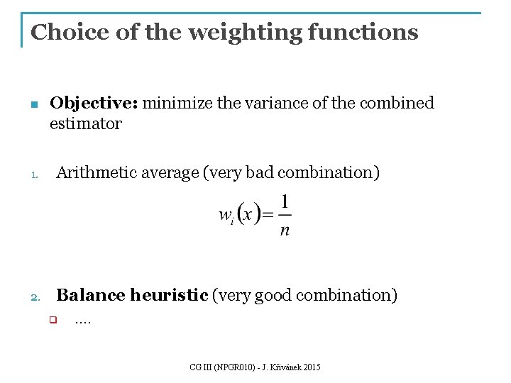
Choice of the weighting functions n Objective: minimize the variance of the combined estimator 1. Arithmetic average (very bad combination) 2. Balance heuristic (very good combination) q …. CG III (NPGR 010) - J. Křivánek 2015

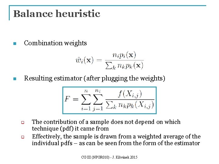
Balance heuristic n Combination weights n Resulting estimator (after plugging the weights) q q The contribution of a sample does not depend on which technique (pdf) it came from Effectively, the sample is drawn from a weighted average of the individual pdfs – as can be seen from the form of the estimator CG III (NPGR 010) - J. Křivánek 2015

Balance heuristic n The balance heuristic is almost optimal q No other weighting has variance much lower than the balance heuristic CG III (NPGR 010) - J. Křivánek 2015

Direct illumination calculation using MIS

Application of MIS to environment light sampling n n Two sampling strategies for generating the incident direction wi 1. BRDF-proportional sampling - pa(wi) 2. Environment map-proportional sampling - pb(wi) Mindlessly plug pa(wi) and pb(wi) into the general formulas above CG III (NPGR 010) - J. Křivánek 2015

MIS 300 + 300 samples EM IS 600 samples BRDF IS 600 samples MIS applied to enviro sampling Diffuse only Ward BRDF, a=0. 2 Ward BRDF, a=0. 05 Ward BRDF, a=0. 01

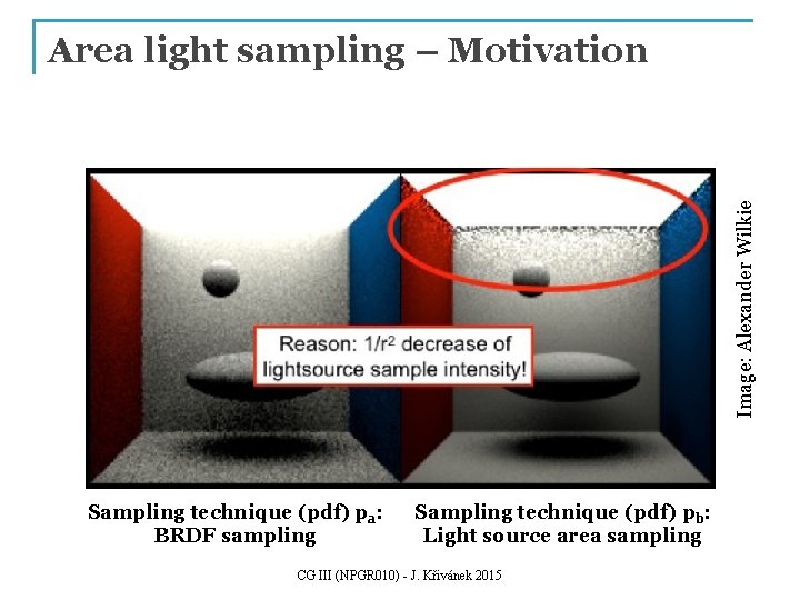
Image: Alexander Wilkie Area light sampling – Motivation Sampling technique (pdf) pa: BRDF sampling Sampling technique (pdf) pb: Light source area sampling CG III (NPGR 010) - J. Křivánek 2015

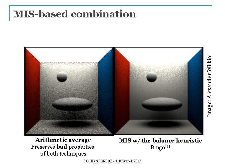
Image: Alexander Wilkie MIS-based combination Arithmetic average Preserves bad properties of both techniques MIS w/ the balance heuristic Bingo!!! CG III (NPGR 010) - J. Křivánek 2015

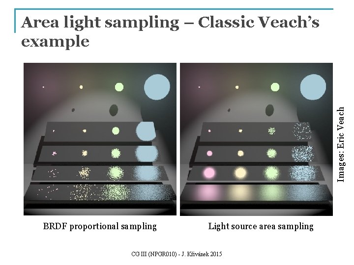
Images: Eric Veach Area light sampling – Classic Veach’s example BRDF proportional sampling Light source area sampling CG III (NPGR 010) - J. Křivánek 2015

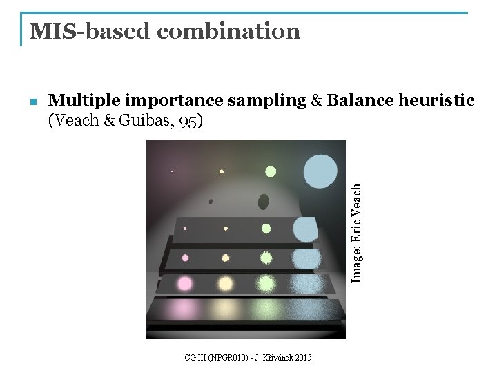
MIS-based combination Multiple importance sampling & Balance heuristic (Veach & Guibas, 95) Image: Eric Veach n CG III (NPGR 010) - J. Křivánek 2015

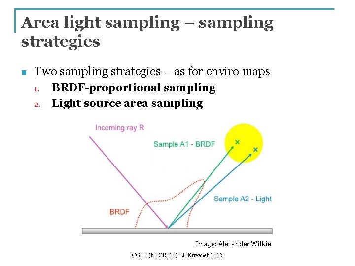
Area light sampling – sampling strategies n Two sampling strategies – as for enviro maps 1. 2. BRDF-proportional sampling Light source area sampling Image: Alexander Wilkie CG III (NPGR 010) - J. Křivánek 2015

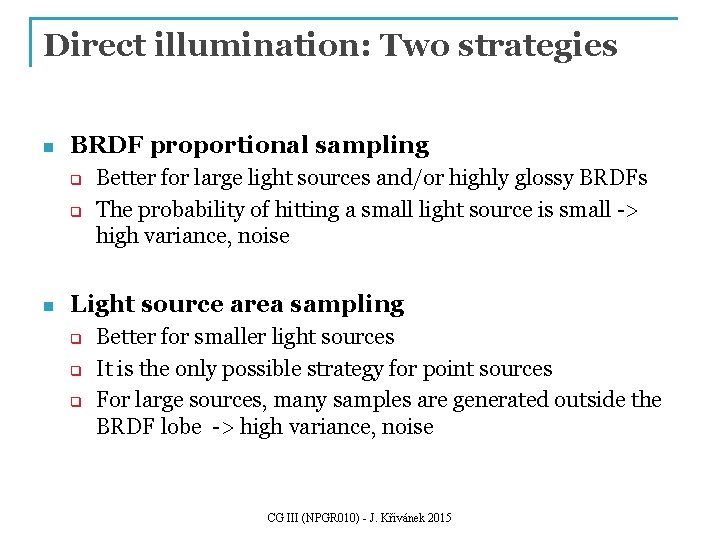
Direct illumination: Two strategies n BRDF proportional sampling q q n Better for large light sources and/or highly glossy BRDFs The probability of hitting a small light source is small -> high variance, noise Light source area sampling q q q Better for smaller light sources It is the only possible strategy for point sources For large sources, many samples are generated outside the BRDF lobe -> high variance, noise CG III (NPGR 010) - J. Křivánek 2015

Direct illumination: Two strategies n Which strategy should we choose? q n Both strategies estimate the same quantity Lr(x, wo) q n Both! A mere sum would estimate 2 x Lr(x, wo) , which is wrong We need a weighted average of the techniques, but how to choose the weights? => MIS CG III (NPGR 010) - J. Křivánek 2015

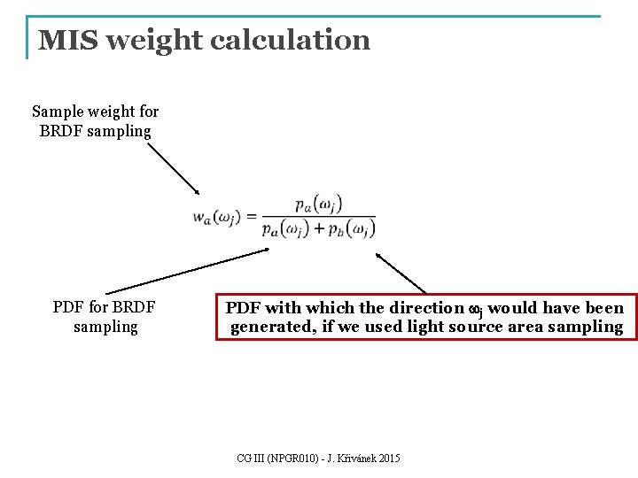
MIS weight calculation Sample weight for BRDF sampling PDF with which the direction wj would have been generated, if we used light source area sampling CG III (NPGR 010) - J. Křivánek 2015

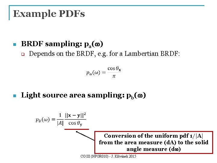
Example PDFs n BRDF sampling: pa(w) q Depends on the BRDF, e. g. for a Lambertian BRDF: n Light source area sampling: pb(w) Conversion of the uniform pdf 1/|A| from the area measure (d. A) to the solid angle measure (dw) CG III (NPGR 010) - J. Křivánek 2015

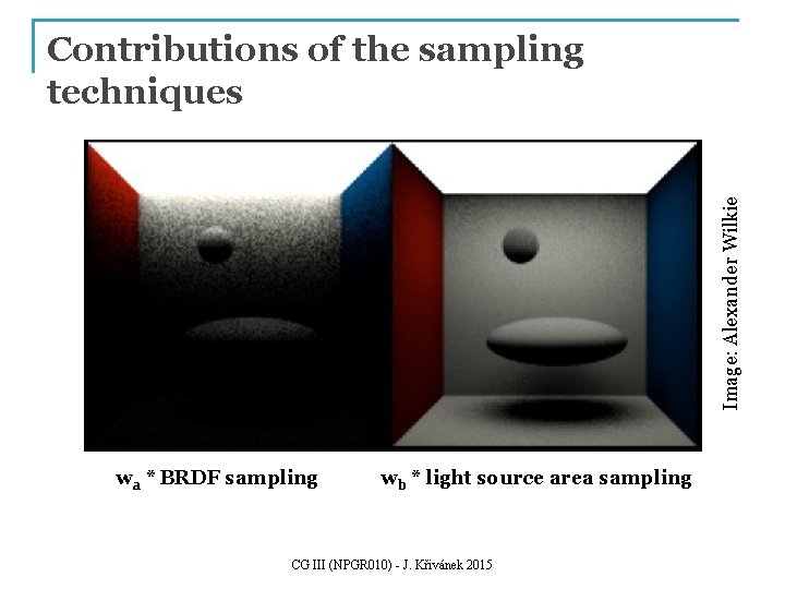
Image: Alexander Wilkie Contributions of the sampling techniques wa * BRDF sampling wb * light source area sampling CG III (NPGR 010) - J. Křivánek 2015

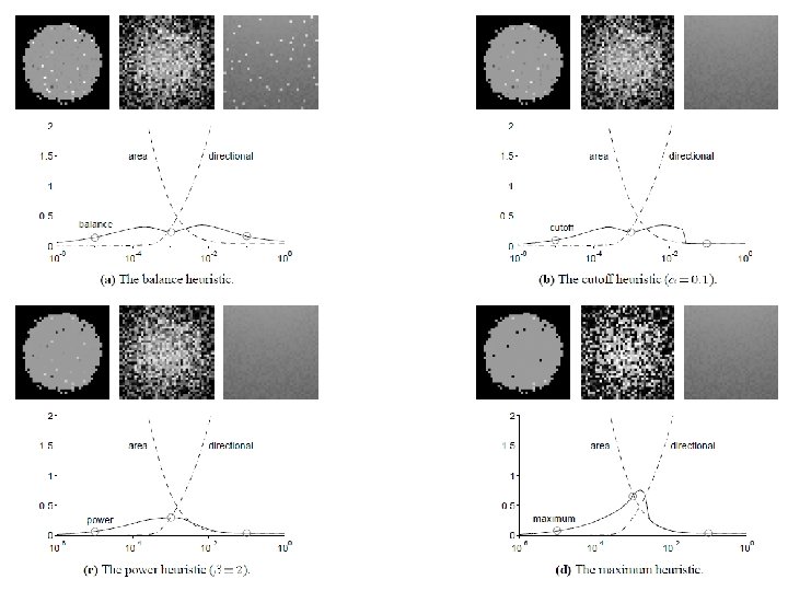
Alternative combination heuristics n “Low variance problems” n Whenever one sampling technique yields a very low variance estimator, balance heuristic can be suboptimal n “Power heuristic” or other heuristics can be better in such a case – see next slide CG III (NPGR 010) - J. Křivánek 2015

CG III (NPGR 010) - J. Křivánek 2015

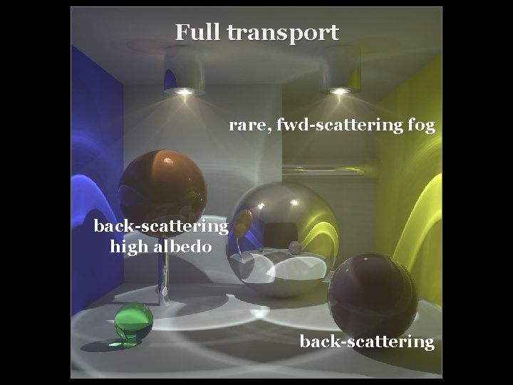
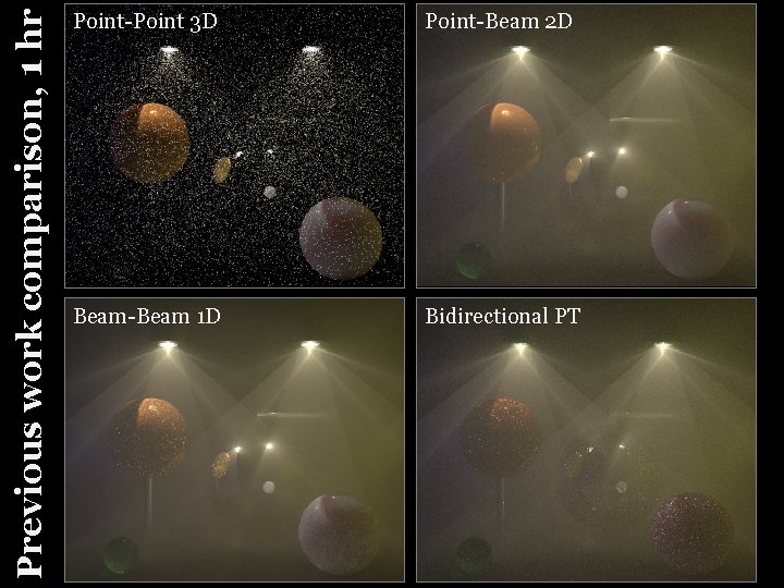
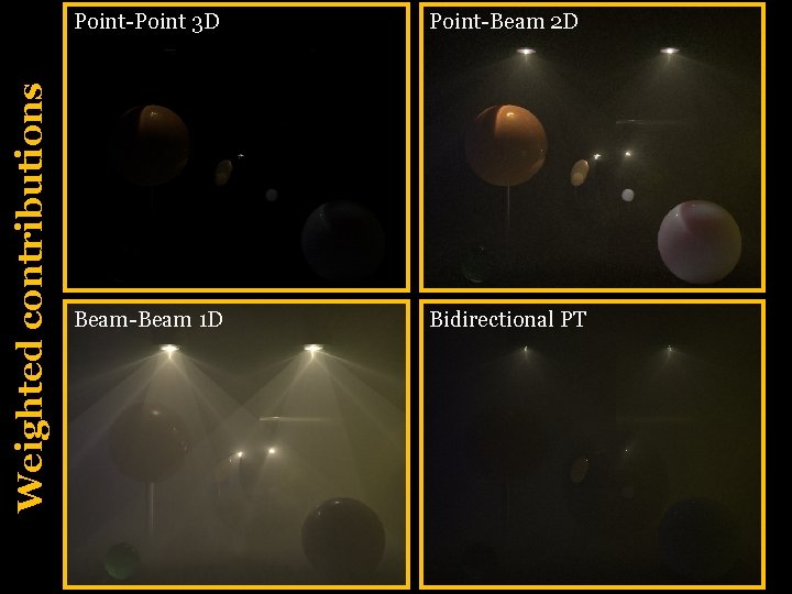
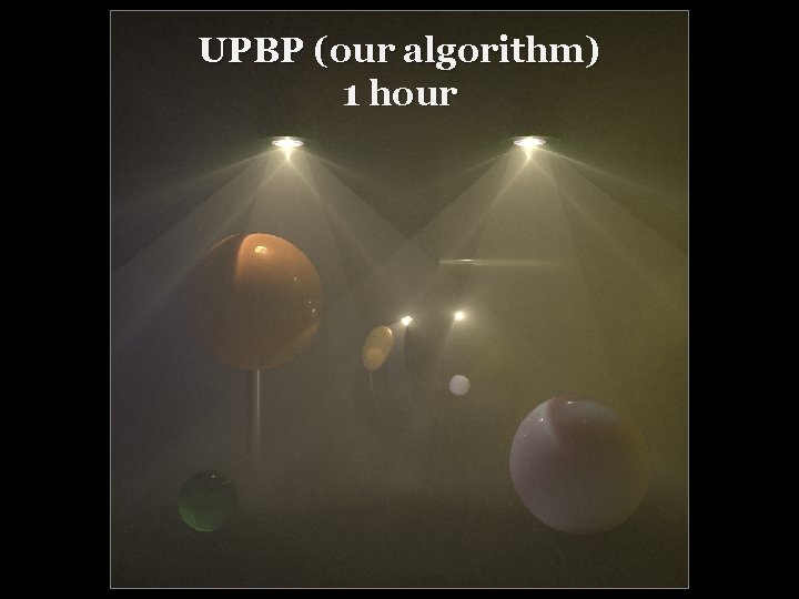
Other examples of MIS applications In the following we apply MIS to combine full path sampling techniques for calculating light transport in participating media.

Full transport rare, fwd-scattering fog back-scattering high albedo back-scattering

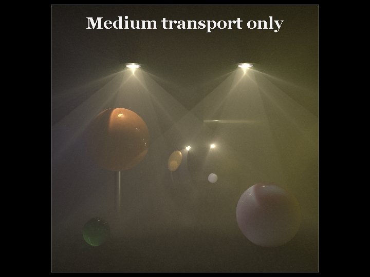
Medium transport only

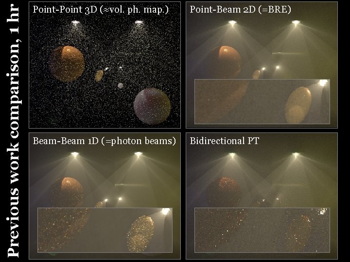
Previous work comparison, 1 hr Point-Point 3 D (≈vol. ph. map. ) Point-Beam 2 D (=BRE) Beam-Beam 1 D (=photon beams) Bidirectional PT

Previous work comparison, 1 hr Point-Point 3 D Point-Beam 2 D Beam-Beam 1 D Bidirectional PT

Weighted contributions Point-Point 3 D Point-Beam 2 D Beam-Beam 1 D Bidirectional PT

UPBP (our algorithm) 1 hour 35