Computer graphics III Monte Carlo integration II Jaroslav
- Slides: 53

Computer graphics III – Monte Carlo integration II Jaroslav Křivánek, MFF UK Jaroslav. Krivanek@mff. cuni. cz

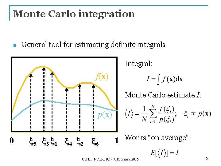
Monte Carlo integration n General tool for estimating definite integrals Integral: f(x) Monte Carlo estimate I: p(x) 0 5 3 1 4 2 6 1 Works “on average”: CG III (NPGR 010) - J. Křivánek 2015 2

Generating samples from a distribution

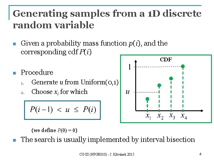
Generating samples from a 1 D discrete random variable n Given a probability mass function p(i), and the corresponding cdf P(i) CDF n Procedure 1. 2. Generate u from Uniform(0, 1) Choose xi for which (we define P(0) = 0) n The search is usually implemented by interval bisection CG III (NPGR 010) - J. Křivánek 2015 4

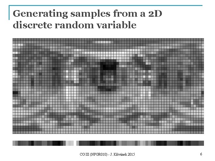
Generating samples from a 2 D discrete random variable n Given a probability mass function p. I, J(i, j) n Option 1: q q Interpret the 2 D PMF as a 1 D vector of probabilities Generate samples as in the 1 D case CG III (NPGR 010) - J. Křivánek 2015 5

Generating samples from a 2 D discrete random variable CG III (NPGR 010) - J. Křivánek 2015 6

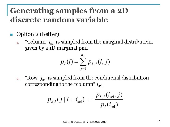
Generating samples from a 2 D discrete random variable n Option 2 (better) 1. 2. “Column” isel is sampled from the marginal distribution, given by a 1 D marginal pmf “Row” jsel is sampled from the conditional distribution corresponding to the “column” isel CG III (NPGR 010) - J. Křivánek 2015 7

Generating samples from a 1 D continuous random variable n Option 1: Transformation method n Option 2: Rejection sampling CG III (NPGR 010) - J. Křivánek 2015 8

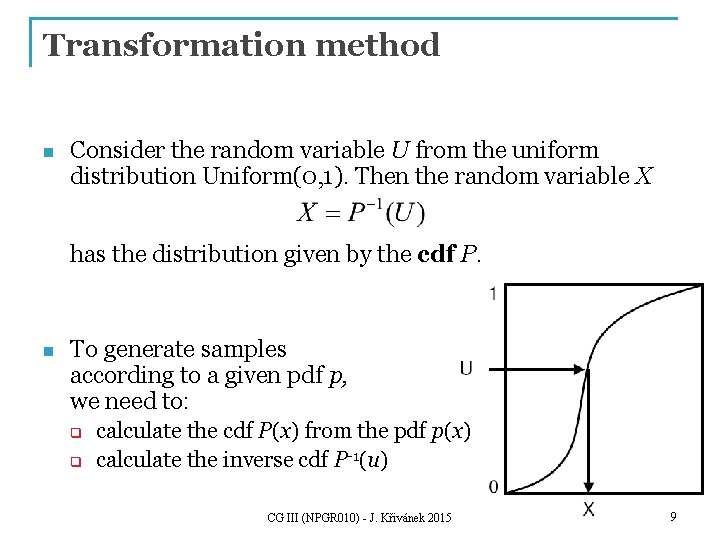
Transformation method n Consider the random variable U from the uniform distribution Uniform(0, 1). Then the random variable X has the distribution given by the cdf P. n To generate samples according to a given pdf p, we need to: q q calculate the cdf P(x) from the pdf p(x) calculate the inverse cdf P-1(u) CG III (NPGR 010) - J. Křivánek 2015 9

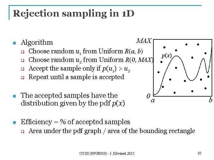
Rejection sampling in 1 D n MAX Algorithm q q Choose random u 1 from Uniform R(a, b) Choose random u 2 from Uniform R(0, MAX) Accept the sample only if p(u 1) > u 2 Repeat until a sample is accepted n The accepted samples have the distribution given by the pdf p(x) n Efficiency = % of accepted samples q 0 p(x) a b Area under the pdf graph / area of the bounding rectangle CG III (NPGR 010) - J. Křivánek 2015 10

Transformation method vs. Rejection sampling n Transformation method Pros n n n Transformation method Cons n n Almost always more efficient than rejection sampling (unless the transformation formula x = P-1(u) turns our extremely complex) Has a constant time complexity and the random number count is known upfront May not be feasible (we may not be able to find the suitable form for x = P-1(u)), but rejection sampling is always applicable as long as we can evaluate the pdf (i. e. rejection sampling is more general) Smart rejection sampling can be very efficient (e. g. the Ziggurat method, see Wikipedia) CG III (NPGR 010) - J. Křivánek 2015 11

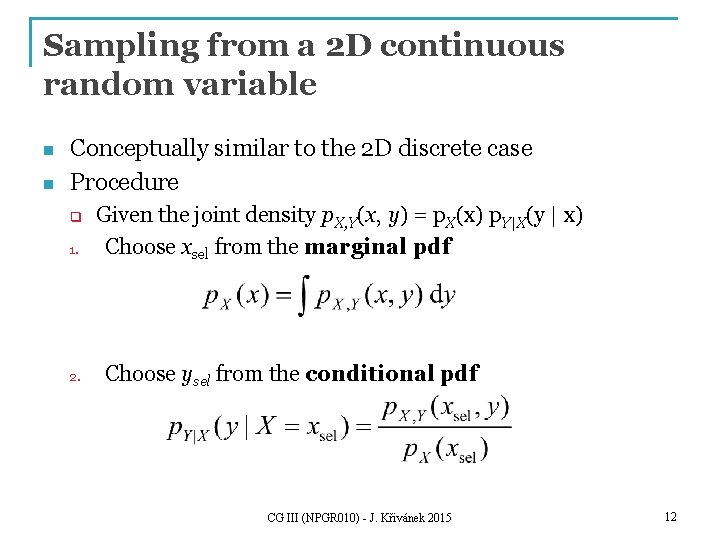
Sampling from a 2 D continuous random variable n n Conceptually similar to the 2 D discrete case Procedure q 1. 2. Given the joint density p. X, Y(x, y) = p. X(x) p. Y|X(y | x) Choose xsel from the marginal pdf Choose ysel from the conditional pdf CG III (NPGR 010) - J. Křivánek 2015 12

Transformation formulas for common cases in light transport n P. Dutré: Global Illumination Compendium, http: //people. cs. kuleuven. be/~philip. dutre/GI/ CG III (NPGR 010) - J. Křivánek 2015 13

Importance sampling from the physically-plausible Phong BRDF n Ray hits a surface with a Phong BRDF. How do we generate the ray for continuing the light path? n Procedure 1. Choose the BRDF component (diffuse reflection, specular reflection, refraction) 2. Sample the chosen component 3. Evaluate the total PDF and BRDF CG III (NPGR 010) - J. Křivánek 2015 14

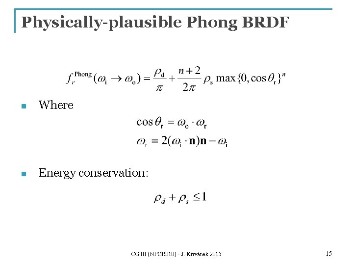
Physically-plausible Phong BRDF n Where n Energy conservation: CG III (NPGR 010) - J. Křivánek 2015 15

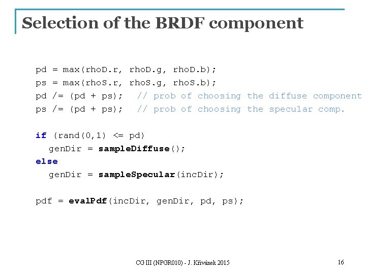
Selection of the BRDF component pd ps = max(rho. D. r, rho. D. g, rho. D. b); = max(rho. S. r, rho. S. g, rho. S. b); /= (pd + ps); // prob of choosing the diffuse component /= (pd + ps); // prob of choosing the specular comp. if (rand(0, 1) <= pd) gen. Dir = sample. Diffuse(); else gen. Dir = sample. Specular(inc. Dir); pdf = eval. Pdf(inc. Dir, gen. Dir, pd, ps); CG III (NPGR 010) - J. Křivánek 2015 16

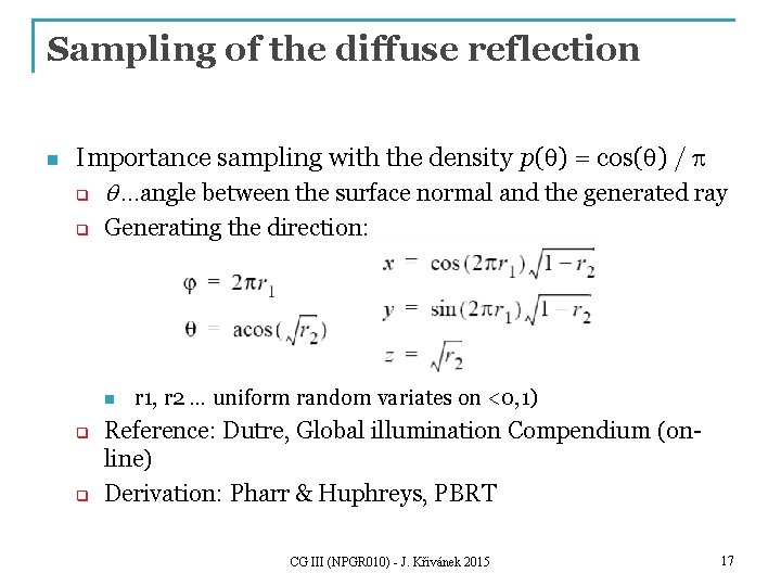
Sampling of the diffuse reflection n Importance sampling with the density p(q) = cos(q) / p q q …angle between the surface normal and the generated ray q Generating the direction: n q q r 1, r 2 … uniform random variates on <0, 1) Reference: Dutre, Global illumination Compendium (online) Derivation: Pharr & Huphreys, PBRT CG III (NPGR 010) - J. Křivánek 2015 17

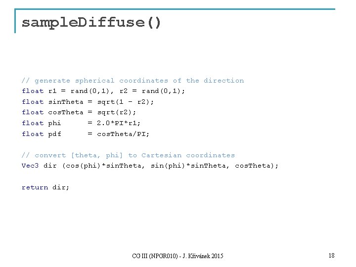
sample. Diffuse() // generate spherical coordinates of the direction float r 1 = rand(0, 1), r 2 = rand(0, 1); float sin. Theta = sqrt(1 – r 2); float cos. Theta = sqrt(r 2); float phi = 2. 0*PI*r 1; float pdf = cos. Theta/PI; // convert [theta, phi] to Cartesian coordinates Vec 3 dir (cos(phi)*sin. Theta, sin(phi)*sin. Theta, cos. Theta); return dir; CG III (NPGR 010) - J. Křivánek 2015 18

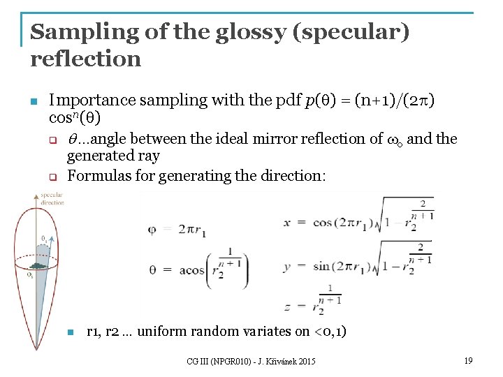
Sampling of the glossy (specular) reflection n Importance sampling with the pdf p(q) = (n+1)/(2 p) cosn(q) q q …angle between the ideal mirror reflection of wo and the q generated ray Formulas for generating the direction: n r 1, r 2 … uniform random variates on <0, 1) CG III (NPGR 010) - J. Křivánek 2015 19

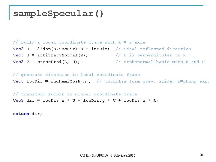
sample. Specular() // build Vec 3 R = Vec 3 U = Vec 3 V = a local coordinate frame with R 2*dot(N, inc. Dir)*N – inc. Dir; // arbitrary. Normal(R); // cross. Prod(R, U); // = z-axis ideal reflected direction U is perpendicular to R orthonormal basis with R and U // generate direction in local coordinate frame Vec 3 loc. Dir = rnd. Hemi. Cos. N(n); // formulas form prev. slide, n=phong exp. // transform loc. Dir to global coordinate frame Vec 3 dir = loc. Dir. x * U + loc. Dir. y * V + loc. Dir. z * R; return dir; CG III (NPGR 010) - J. Křivánek 2015 20

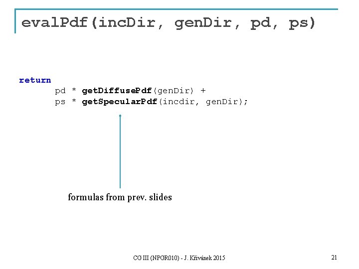
eval. Pdf(inc. Dir, gen. Dir, pd, ps) return pd * get. Diffuse. Pdf(gen. Dir) + ps * get. Specular. Pdf(incdir, gen. Dir); formulas from prev. slides CG III (NPGR 010) - J. Křivánek 2015 21

Variance reduction methods for MC estimators

Variance reduction methods n Importance sampling q The most commonly used method in light transport (most often we use BRDF-proportional importance sampling) n Control variates n Improved sample distribution q q Stratification quasi-Monte Carlo (QMC) CG III (NPGR 010) - J. Křivánek 2015 23

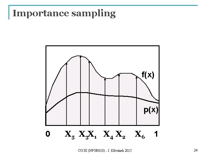
Importance sampling f(x) p(x) 0 X 5 X 3 X 1 X 4 X 2 CG III (NPGR 010) - J. Křivánek 2015 X 6 1 24

Importance sampling n Parts of the integration domain with high value of the integrand f are more important q n Importance sampling places samples preferentially to these areas q n Samples from these areas have higher impact on the result I. e. the pdf p is “similar” to the integrand f Decreases variance while keeping unbiasedness CG III (NPGR 010) - J. Křivánek 2015 25

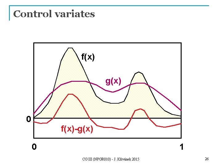
Control variates f(x) g(x) 0 f(x)-g(x) 0 1 CG III (NPGR 010) - J. Křivánek 2015 26

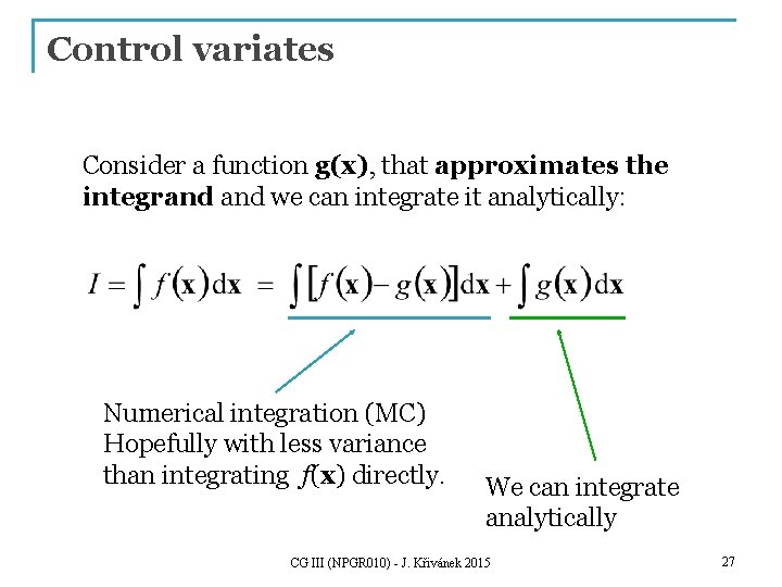
Control variates Consider a function g(x), that approximates the integrand we can integrate it analytically: Numerical integration (MC) Hopefully with less variance than integrating f(x) directly. We can integrate analytically CG III (NPGR 010) - J. Křivánek 2015 27

Control variates vs. Importance sampling n Importance sampling q n Control variates q n Advantageous whenever the function, according to which we can generate samples, appears in the integrand as a multiplicative factor (e. g. BRDF in the reflection equation). Better if the function that we can integrate analytically appears in the integrand as an additive term. This is why in light transport, we almost always use importance sampling and almost never control variates. CG III (NPGR 010) - J. Křivánek 2015 28

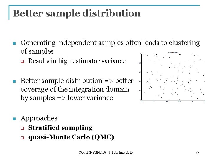
Better sample distribution n Generating independent samples often leads to clustering of samples q Results in high estimator variance n Better sample distribution => better coverage of the integration domain by samples => lower variance n Approaches q q Stratified sampling quasi-Monte Carlo (QMC) CG III (NPGR 010) - J. Křivánek 2015 29

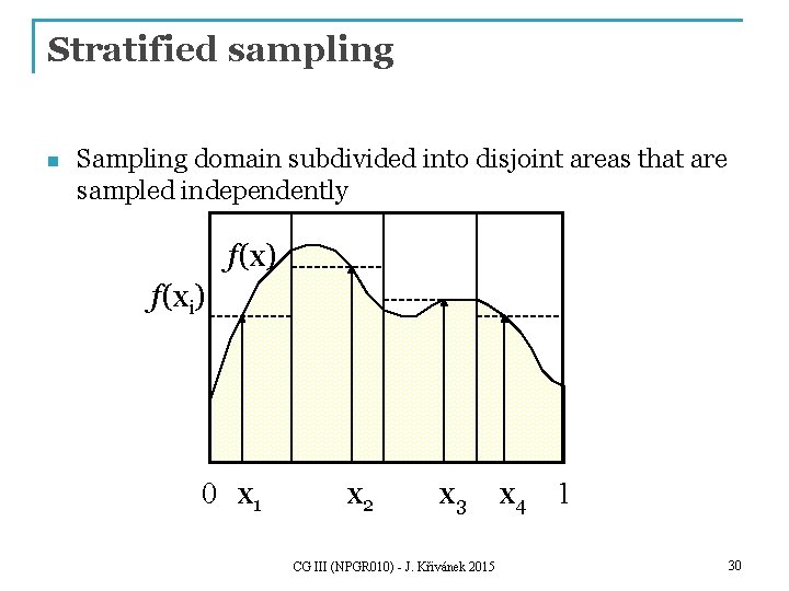
Stratified sampling n Sampling domain subdivided into disjoint areas that are sampled independently f(x) f(xi) 0 x 1 x 2 x 3 CG III (NPGR 010) - J. Křivánek 2015 x 4 1 30

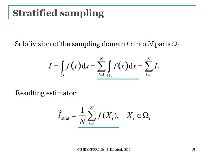
Stratified sampling Subdivision of the sampling domain W into N parts Wi: Resulting estimator: CG III (NPGR 010) - J. Křivánek 2015 31

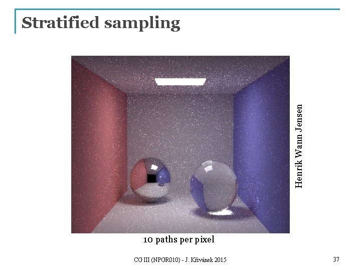
Stratified sampling n Suppresses sample clustering n Reduces estimator variance q n Variance is provably less than or equal to the variance of a regular secondary estimator Very effective in low dimension q Effectiveness deteriorates for high-dimensional integrands CG III (NPGR 010) - J. Křivánek 2015 32

How to subdivide the interval? n Uniform subdivision of the interval q Natural approach for a completely unknown integrand f n If we know at least roughly the shape of the integrand f, we aim for a subdivision with the lowest possible variance on the sub-domains n Subdivision of a d-dimensional interval leads to Nd samples q A better approach in high dimension is N-rooks sampling CG III (NPGR 010) - J. Křivánek 2015 33

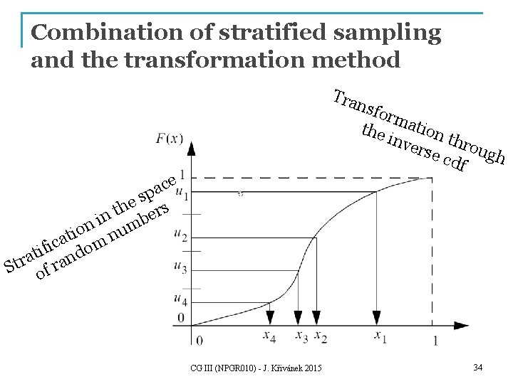
Combination of stratified sampling and the transformation method Tra nsfo rma tion the inve thro rse u cdf gh ce a sp e th ers n i mb n io nu t a c om i f i at and r t S of r CG III (NPGR 010) - J. Křivánek 2015 34

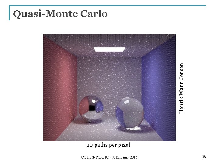
Quasi-Monte Carlo methods (QMC) n Use of strictly deterministic sequences instead of (pseudo -)random numbers n Pseudo-random numbers replaced by low-discrepancy sequences n Everything works as in regular MC, but the underlying math is different (nothing is random so the math cannot be built on probability theory) CG III (NPGR 010) - J. Křivánek 2015 35

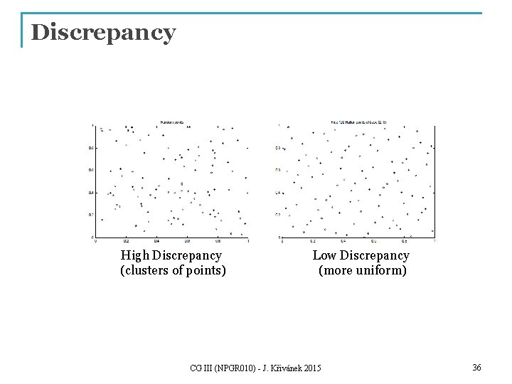
Discrepancy High Discrepancy (clusters of points) Low Discrepancy (more uniform) CG III (NPGR 010) - J. Křivánek 2015 36

Henrik Wann Jensen Stratified sampling 10 paths per pixel CG III (NPGR 010) - J. Křivánek 2015 37

Henrik Wann Jensen Quasi-Monte Carlo 10 paths per pixel CG III (NPGR 010) - J. Křivánek 2015 38

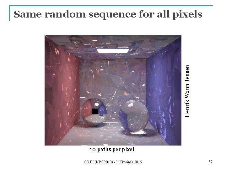
Henrik Wann Jensen Same random sequence for all pixels 10 paths per pixel CG III (NPGR 010) - J. Křivánek 2015 39

Image-based lighting

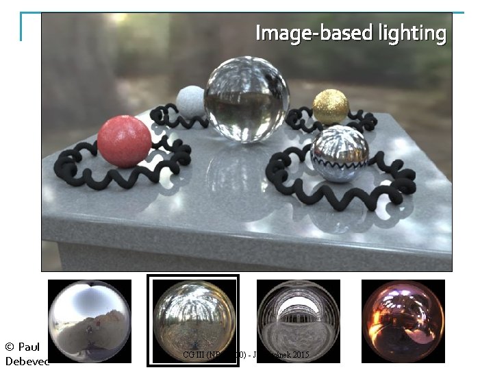
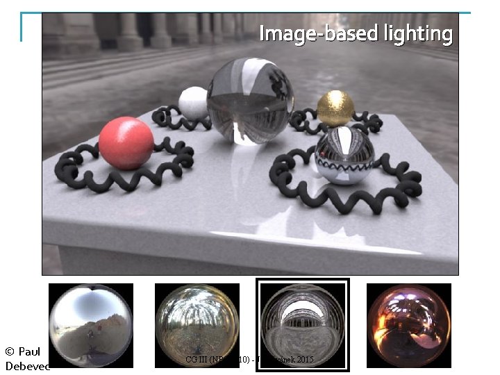
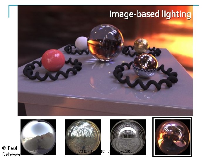
Image-based lighting n Introduced by Paul Debevec (Siggraph 98) n Routinely used for special effects in films & games CG III (NPGR 010) 41 - J. Křivánek 2015

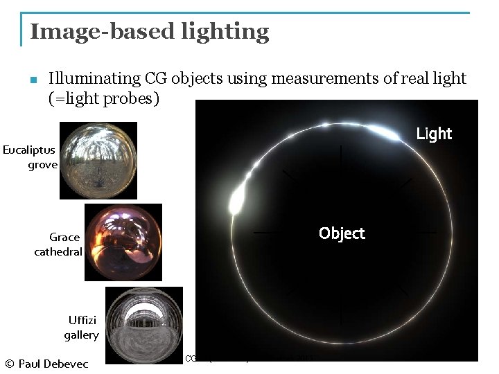
Image-based lighting n Illuminating CG objects using measurements of real light (=light probes) Light Eucaliptus grove Object Grace cathedral Uffizi gallery © Paul Debevec CG III (NPGR 010) 42 - J. Křivánek 2015

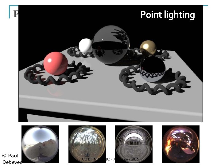
Point Light Source © Paul Debevec CG III (NPGR 010) 43 - J. Křivánek 2015 Point lighting

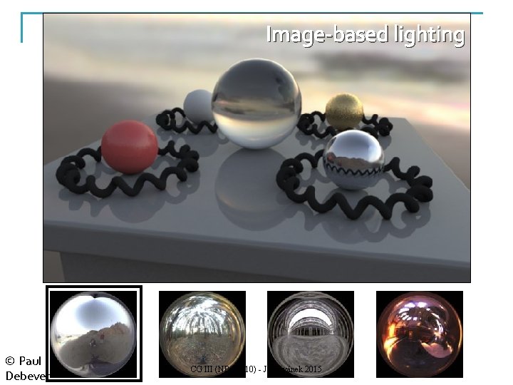
Image-based lighting © Paul Debevec CG III (NPGR 010) 44 - J. Křivánek 2015

Image-based lighting © Paul Debevec CG III (NPGR 010) 45 - J. Křivánek 2015

Image-based lighting © Paul Debevec CG III (NPGR 010) 46 - J. Křivánek 2015

Image-based lighting © Paul Debevec CG III (NPGR 010) 47 - J. Křivánek 2015

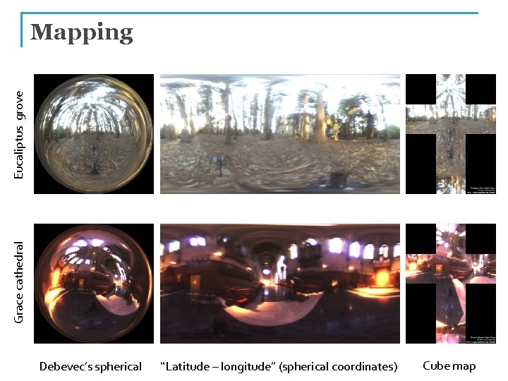
Grace cathedral Eucaliptus grove Mapping Debevec’s spherical “Latitude – longitude” (spherical coordinates) Cube map

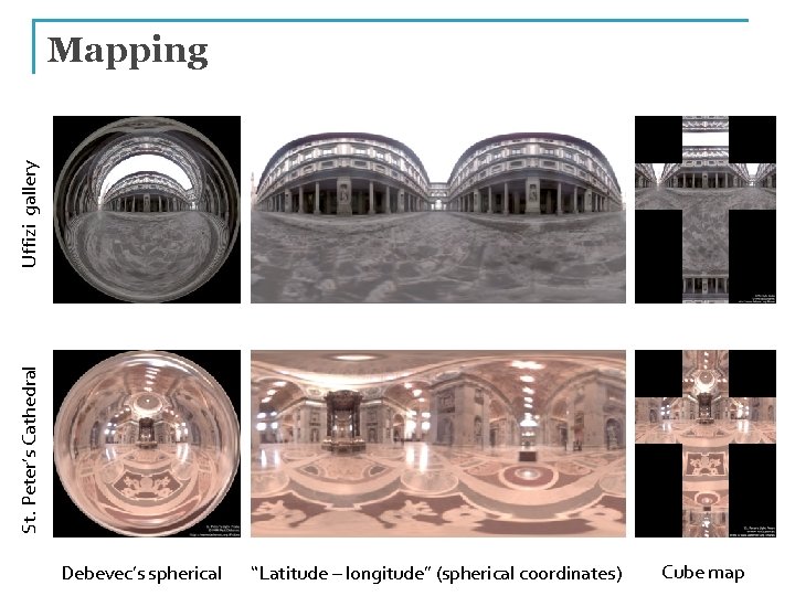
St. Peter’s Cathedral Uffizi gallery Mapping Debevec’s spherical “Latitude – longitude” (spherical coordinates) Cube map

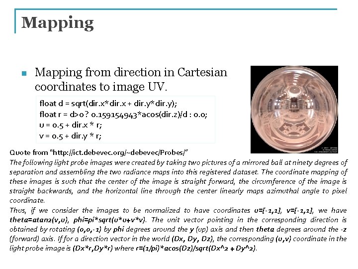
Mapping n Mapping from direction in Cartesian coordinates to image UV. float d = sqrt(dir. x*dir. x + dir. y*dir. y); float r = d>0 ? 0. 159154943*acos(dir. z)/d : 0. 0; u = 0. 5 + dir. x * r; v = 0. 5 + dir. y * r; Quote from “http: //ict. debevec. org/~debevec/Probes/” The following light probe images were created by taking two pictures of a mirrored ball at ninety degrees of separation and assembling the two radiance maps into this registered dataset. The coordinate mapping of these images is such that the center of the image is straight forward, the circumference of the image is straight backwards, and the horizontal line through the center linearly maps azimuthal angle to pixel coordinate. Thus, if we consider the images to be normalized to have coordinates u=[-1, 1], v=[-1, 1], we have theta=atan 2(v, u), phi=pi*sqrt(u*u+v*v). The unit vector pointing in the corresponding direction is obtained by rotating (0, 0, -1) by phi degrees around the y (up) axis and then theta degrees around the -z (forward) axis. If for a direction vector in the world (Dx, Dy, Dz), the corresponding (u, v) coordinate in the light probe image is (Dx*r, Dy*r) where r=(1/pi)*acos(Dz)/sqrt(Dx^2 + Dy^2). 50

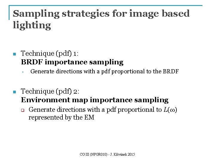
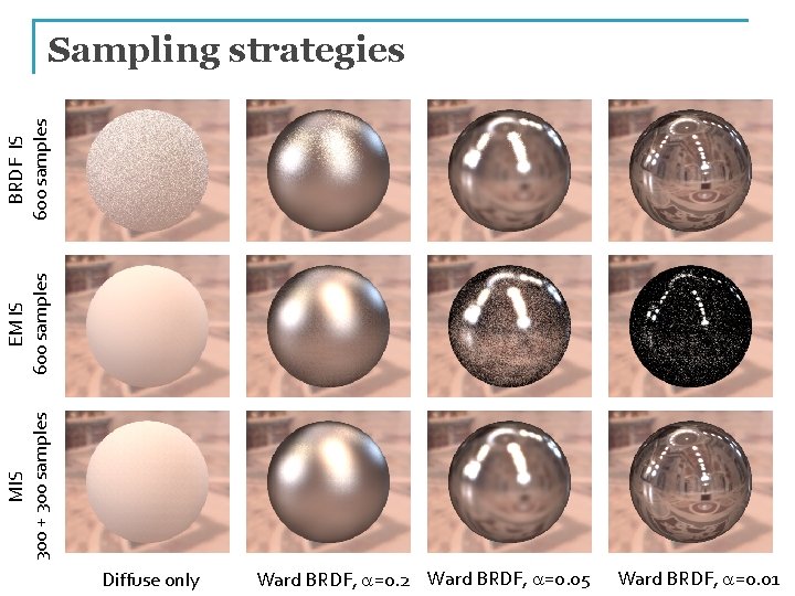
Sampling strategies for image based lighting n Technique (pdf) 1: BRDF importance sampling • n Generate directions with a pdf proportional to the BRDF Technique (pdf) 2: Environment map importance sampling q Generate directions with a pdf proportional to L(w) represented by the EM CG III (NPGR 010) 51 - J. Křivánek 2015

MIS 300 + 300 samples EM IS 600 samples BRDF IS 600 samples Sampling strategies Diffuse only Ward BRDF, a=0. 2 Ward BRDF, a=0. 05 Ward BRDF, a=0. 01

Sampling according to the environment map luminance n Luminance of the environment map defines the sampling pdf on the unit sphere n For details, see PBRT CG III (NPGR 010) - J. Křivánek 2015 53