Computer Graphics Fall 2005 COMS 4160 Lecture 7

Computer Graphics (Fall 2005) COMS 4160, Lecture 7: Curves 2 http: //www. cs. columbia. edu/~cs 4160

To Do § Start on HW 2 (cannot be done at last moment) This (and previous) lecture should have all information need § Start thinking about partners for HW 3 and HW 4 § Remember though, that HW 2 is done individually § Your submission of HW 2 must include partner for HW 3

Outline of Unit § Bezier curves (last time) § de. Casteljau algorithm, explicit, matrix (last time) § Polar form labeling (blossoms) § B-spline curves § Not well covered in textbooks (especially as taught here). Main reference will be lecture notes. If you do want a printed ref, handouts from CAGD, Seidel

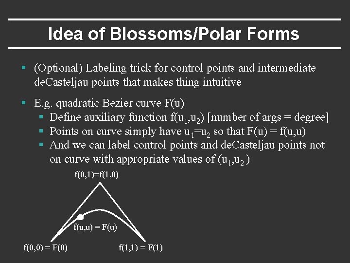
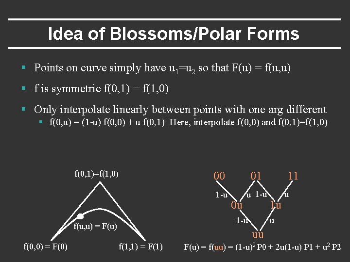
Idea of Blossoms/Polar Forms § (Optional) Labeling trick for control points and intermediate de. Casteljau points that makes thing intuitive § E. g. quadratic Bezier curve F(u) § Define auxiliary function f(u 1, u 2) [number of args = degree] § Points on curve simply have u 1=u 2 so that F(u) = f(u, u) § And we can label control points and de. Casteljau points not on curve with appropriate values of (u 1, u 2 ) f(0, 1)=f(1, 0) f(u, u) = F(u) f(0, 0) = F(0) f(1, 1) = F(1)

Idea of Blossoms/Polar Forms § Points on curve simply have u 1=u 2 so that F(u) = f(u, u) § f is symmetric f(0, 1) = f(1, 0) § Only interpolate linearly between points with one arg different § f(0, u) = (1 -u) f(0, 0) + u f(0, 1) Here, interpolate f(0, 0) and f(0, 1)=f(1, 0) 01 1 -u u 1 -u 0 u 1 -u f(u, u) = F(u) f(0, 0) = F(0) 00 11 1 u u u uu f(1, 1) = F(1) F(u) = f(uu) = (1 -u)2 P 0 + 2 u(1 -u) P 1 + u 2 P 2

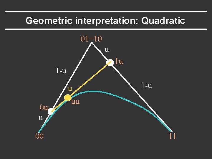
Geometric interpretation: Quadratic 01=10 u 1 u 1 -u u 00 1 -u uu 11

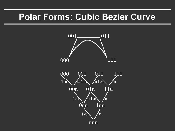
Polar Forms: Cubic Bezier Curve 001 011 111 000 001 011 1 -u u 00 u 11 u 01 u 1 -u u 0 uu 1 -u u uuu

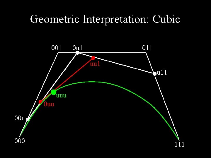
Geometric Interpretation: Cubic 001 0 u 1 011 uu 1 u 11 uuu 00 u 000 111

Why Polar Forms? § Simple mnemonic: which points to interpolate and how in de. Casteljau algorithm § Easy to see how to subdivide Bezier curve (next) which is useful for drawing recursively § Generalizes to arbitrary spline curves (just label control points correctly instead of 00 01 11 for Bezier) § Easy for many analyses (beyond scope of course)

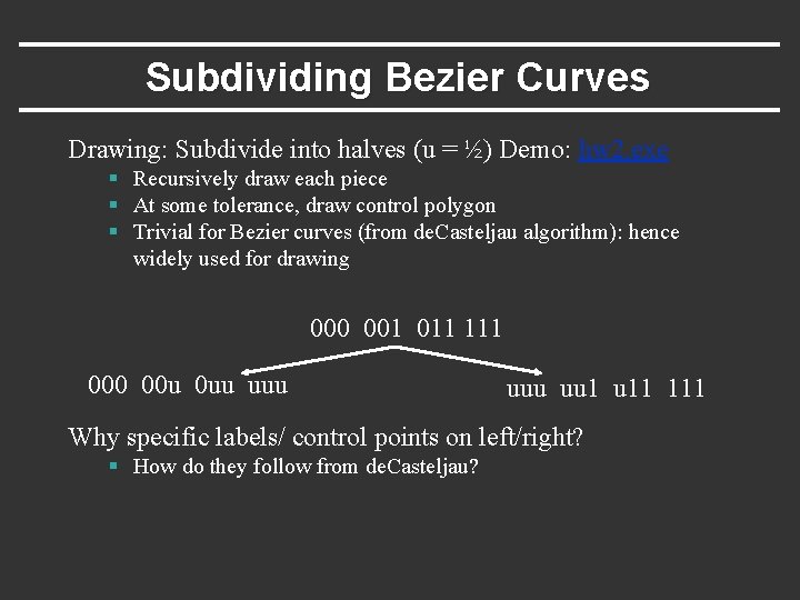
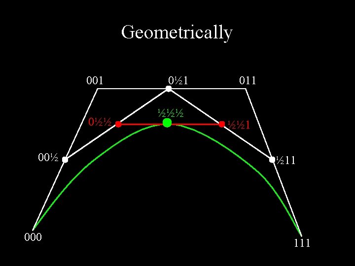
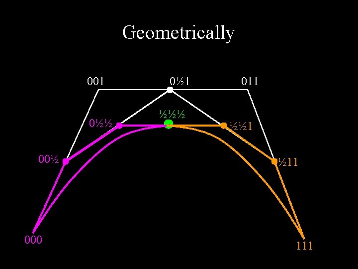
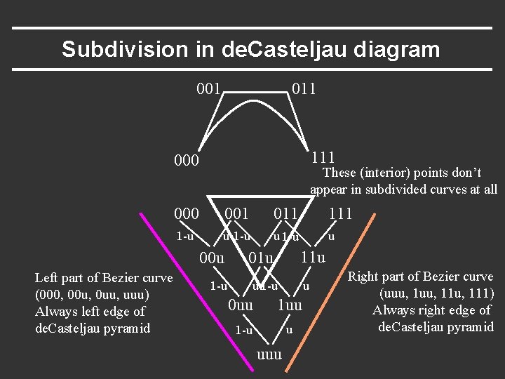
Subdividing Bezier Curves Drawing: Subdivide into halves (u = ½) Demo: hw 2. exe § Recursively draw each piece § At some tolerance, draw control polygon § Trivial for Bezier curves (from de. Casteljau algorithm): hence widely used for drawing 000 001 011 111 000 00 u 0 uu uuu uu 1 u 11 111 Why specific labels/ control points on left/right? § How do they follow from de. Casteljau?

Geometrically 001 0½½ 000 0½ 1 ½½½ 011 ½½ 1 ½ 11 111

Geometrically 001 0½½ 000 0½ 1 ½½½ 011 ½½ 1 ½ 11 111

Subdivision in de. Casteljau diagram 001 011 111 000 These (interior) points don’t appear in subdivided curves at all 000 001 011 1 -u u 00 u Left part of Bezier curve (000, 00 u, 0 uu, uuu) Always left edge of de. Casteljau pyramid 11 u 01 u 1 -u u 0 uu 1 -u u uuu Right part of Bezier curve (uuu, 11 u, 111) Always right edge of de. Casteljau pyramid

Summary for HW 2 § Bezier 2 (Bezier discussed last time) § Given arbitrary degree Bezier curve, recursively subdivide for some levels, then draw control polygon hw 2. exe § Generate de. Casteljau diagram; recursively call a routine with left edge and right edge of this diagram § You are given some code structure; you essentially just need to compute appropriate control points for left, right

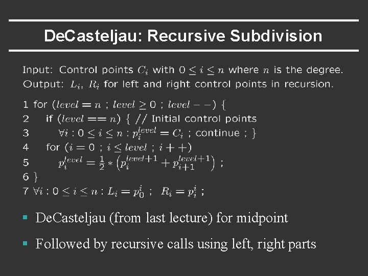
De. Casteljau: Recursive Subdivision § De. Casteljau (from last lecture) for midpoint § Followed by recursive calls using left, right parts

Outline of Unit § Bezier curves (last time) § de. Casteljau algorithm, explicit, matrix (last time) § Polar form labeling (blossoms) § B-spline curves § Not well covered in textbooks (especially as taught here). Main reference will be lecture notes. If you do want a printed ref, handouts from CAGD, Seidel

Bezier: Disadvantages § Single piece, no local control (move a control point, whole curve changes) hw 2. exe § Complex shapes: can be very high degree, difficult § In practice, combine many Bezier curve segments § But only position continuous at join since Bezier curves interpolate end-points (which match at segment boundaries) § Unpleasant derivative (slope) discontinuities at end-points § Can you see why this is an issue?

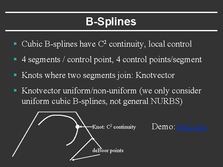
B-Splines § Cubic B-splines have C 2 continuity, local control § 4 segments / control point, 4 control points/segment § Knots where two segments join: Knotvector § Knotvector uniform/non-uniform (we only consider uniform cubic B-splines, not general NURBS) Knot: C 2 continuity de. Boor points Demo: hw 2. exe

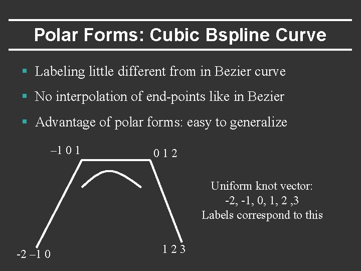
Polar Forms: Cubic Bspline Curve § Labeling little different from in Bezier curve § No interpolation of end-points like in Bezier § Advantage of polar forms: easy to generalize – 1 012 Uniform knot vector: -2, -1, 0, 1, 2 , 3 Labels correspond to this -2 – 1 0 123

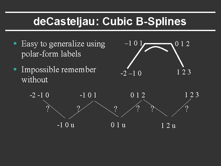
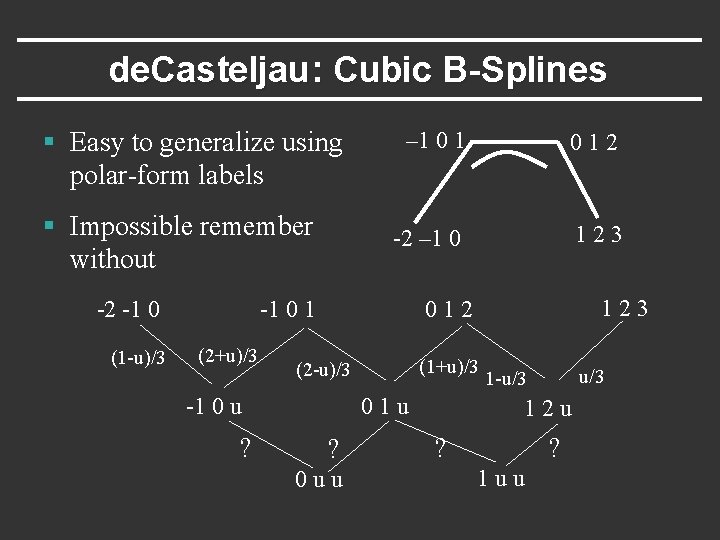
de. Casteljau: Cubic B-Splines § Easy to generalize using polar-form labels § Impossible remember without -2 -1 0 – 1 012 -2 – 1 0 123 ? ? -1 0 u 123 012 -1 0 1 ? 01 u ? ? ? 12 u

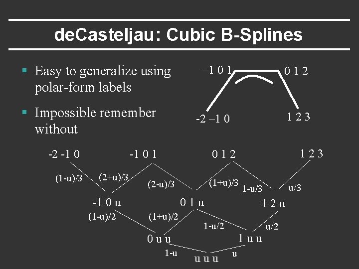
de. Casteljau: Cubic B-Splines § Easy to generalize using polar-form labels § Impossible remember without -2 -1 0 (1 -u)/3 – 1 012 -2 – 1 0 123 (2+u)/3 (1+u)/3 (2 -u)/3 -1 0 u ? 123 012 -1 0 1 01 u ? 0 uu u/3 1 -u/3 12 u ? ? 1 uu

de. Casteljau: Cubic B-Splines § Easy to generalize using polar-form labels § Impossible remember without -2 -1 0 (1 -u)/3 – 1 012 -2 – 1 0 123 (2+u)/3 (1+u)/3 (2 -u)/3 -1 0 u (1 -u)/2 123 012 -1 0 1 01 u (1+u)/2 12 u 1 -u/2 1 uu 0 uu 1 -u uuu u/3 1 -u/3 u u/2

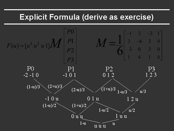
Explicit Formula (derive as exercise) P 0 -2 -1 0 (1 -u)/3 P 2 P 1 (1+u)/3 (2 -u)/3 -1 0 u (1 -u)/2 123 012 -1 0 1 (2+u)/3 P 3 01 u (1+u)/2 12 u 1 -u/2 1 uu 0 uu 1 -u uuu u/3 1 -u/3 u u/2

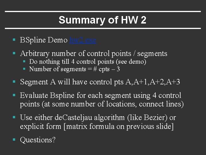
Summary of HW 2 § BSpline Demo hw 2. exe § Arbitrary number of control points / segments § Do nothing till 4 control points (see demo) § Number of segments = # cpts – 3 § Segment A will have control pts A, A+1, A+2, A+3 § Evaluate Bspline for each segment using 4 control points (at some number of locations, connect lines) § Use either de. Casteljau algorithm (like Bezier) or explicit form [matrix formula on previous slide] § Questions?