Computer Graphics Chapter 3 First Lecture TwoDimensional Graphics

Computer Graphics Chapter 3 First Lecture

Two-Dimensional Graphics

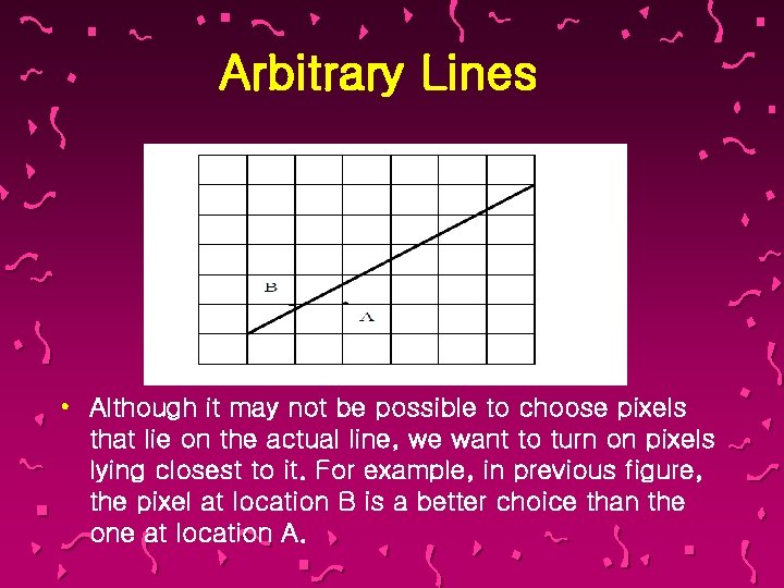
Arbitrary Lines Drawing lines with arbitrary slope creates several problems, such as: 1 - The display screen can be illuminated only at pixels locations; therefore a raster scan display has a staircase effect that only approximates the actual line as shown in figure below: •

Arbitrary Lines • Although it may not be possible to choose pixels that lie on the actual line, we want to turn on pixels lying closest to it. For example, in previous figure, the pixel at location B is a better choice than the one at location A.

Arbitrary Lines • 2 - Determining the closest (best) pixels is not easy. Different algorithms calculate different pixels to make up the approximating line. • The choice of algorithm depends on: • 1 - The speed of line generation. • 2 - The appearance of the line. • Therefore, to understand these criteria better let's look at several different line generating algorithms.

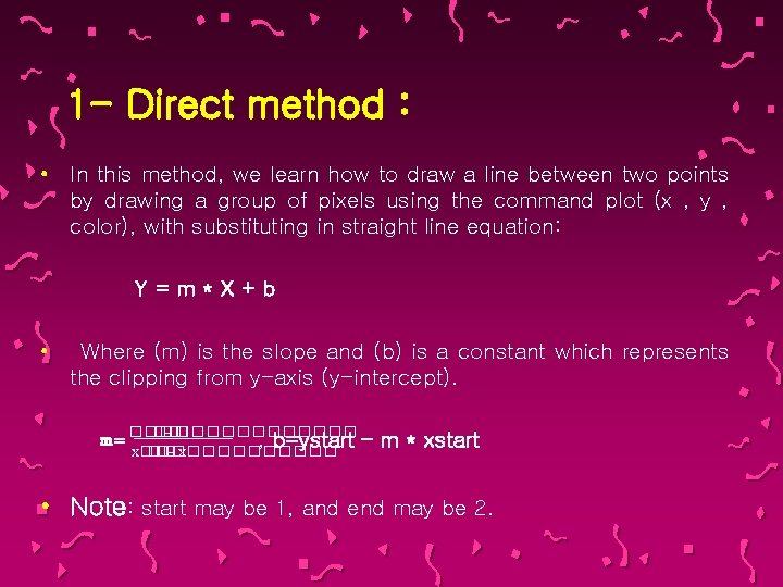
1 - Direct method : • In this method, we learn how to draw a line between two points by drawing a group of pixels using the command plot (x , y , color), with substituting in straight line equation: Y=m*X+b • Where (m) is the slope and (b) is a constant which represents the clipping from y-axis (y-intercept). �� �� – ������ m= ���� , b=ystart – x�� �� �� – x����� m * xstart • Note: start may be 1, and end may be 2.

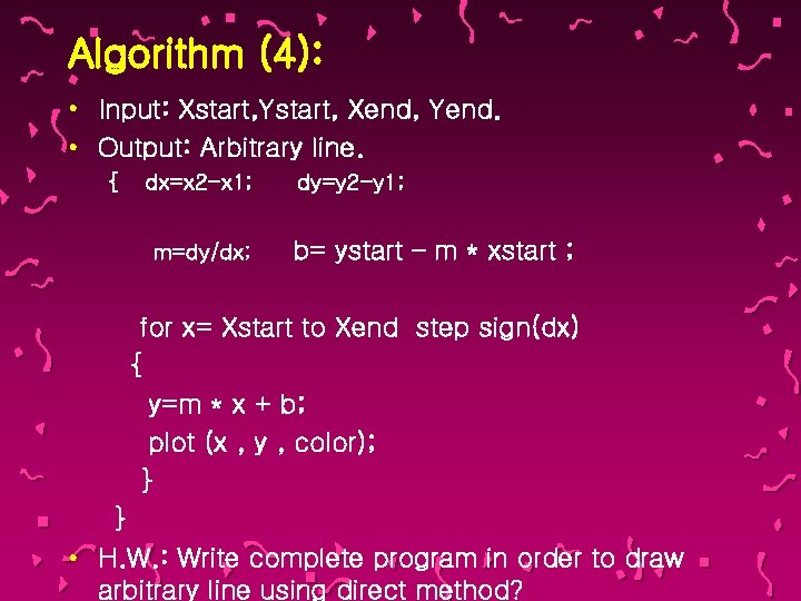
Algorithm (4): • Input: Xstart, Ystart, Xend, Yend. • Output: Arbitrary line. { dx=x 2 -x 1; m=dy/dx; dy=y 2 -y 1; b= ystart – m * xstart ; for x= Xstart to Xend step sign(dx) { y=m * x + b; plot (x , y , color); } } • H. W. : Write complete program in order to draw arbitrary line using direct method?

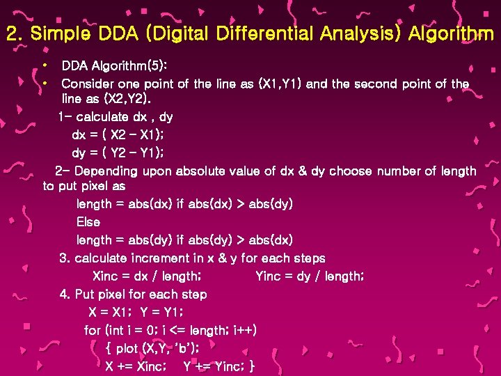
2. Simple DDA (Digital Differential Analysis) Algorithm • • DDA Algorithm(5): Consider one point of the line as (X 1, Y 1) and the second point of the line as (X 2, Y 2). 1 - calculate dx , dy dx = ( X 2 – X 1); dy = ( Y 2 – Y 1); 2 - Depending upon absolute value of dx & dy choose number of length to put pixel as length = abs(dx) if abs(dx) > abs(dy) Else length = abs(dy) if abs(dy) > abs(dx) 3. calculate increment in x & y for each steps Xinc = dx / length; Yinc = dy / length; 4. Put pixel for each step X = X 1; Y = Y 1; for (int i = 0; i <= length; i++) { plot (X, Y, ’b’); X += Xinc; Y += Yinc; }

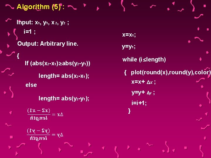
Algorithm (5) : Input: x 1, y 1, x 2, y 2 ; i=1 ; x=x 1; Output: Arbitrary line. { If (abs(x 2 -x 1) ³ abs(y 2 -y 1)) length= abs(x 2 -x 1); y=y 1; while (i £ length) { plot(round(x), round(y), color); x=x+ Dx ; else y=y+ length= abs(y 2 -y 1); i=i+1; } Dy ;

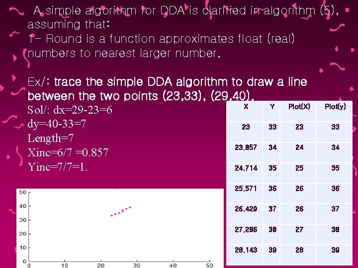
A simple algorithm for DDA is clarified in algorithm (5), assuming that: 1 - Round is a function approximates float (real) numbers to nearest larger number. Ex/: trace the simple DDA algorithm to draw a line between the two points (23, 33), (29, 40). X Y Plot(X) Sol/: dx=29 -23=6 dy=40 -33=7 23 33 23 Length=7 23. 857 34 24 Xinc=6/7 =0. 857 24. 714 35 25 Yinc=7/7=1. Plot(y) 33 34 35 25. 571 36 26. 429 37 26 37 27. 286 38 27 38 28. 143 39 28 39

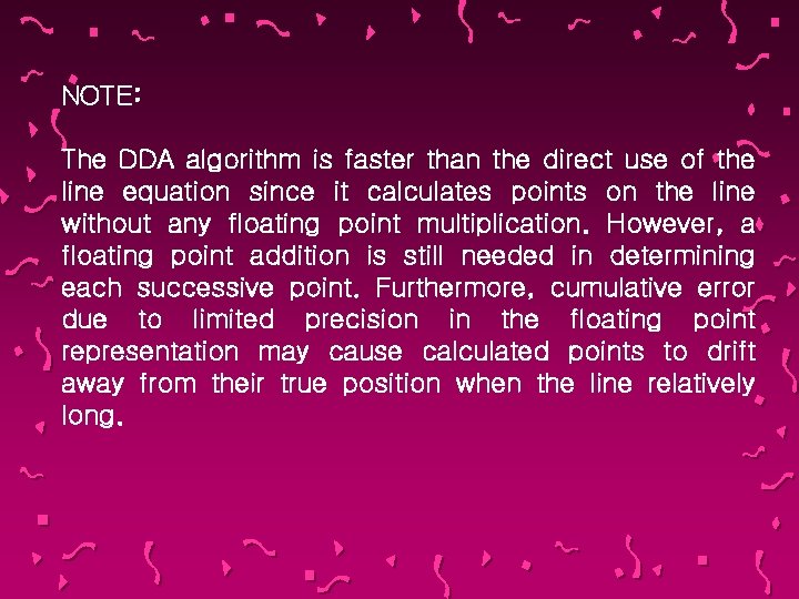
NOTE: The DDA algorithm is faster than the direct use of the line equation since it calculates points on the line without any floating point multiplication. However, a floating point addition is still needed in determining each successive point. Furthermore, cumulative error due to limited precision in the floating point representation may cause calculated points to drift away from their true position when the line relatively long.

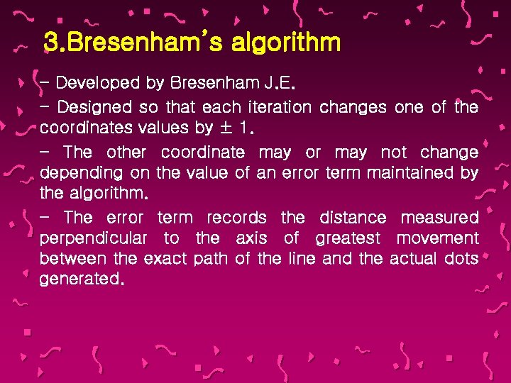
3. Bresenham’s algorithm - Developed by Bresenham J. E. - Designed so that each iteration changes one of the coordinates values by ± 1. - The other coordinate may or may not change depending on the value of an error term maintained by the algorithm. - The error term records the distance measured perpendicular to the axis of greatest movement between the exact path of the line and the actual dots generated.

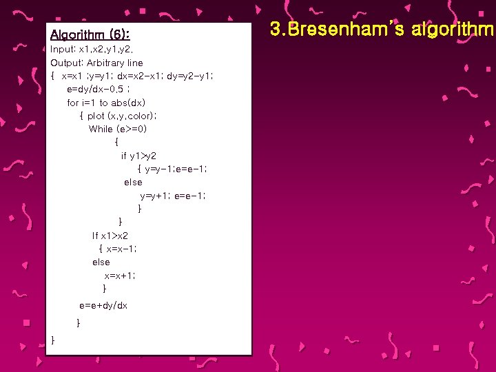
Algorithm (6): Input: x 1, x 2, y 1, y 2. Output: Arbitrary line { x=x 1 ; y=y 1; dx=x 2 -x 1; dy=y 2 -y 1; e=dy/dx-0. 5 ; for i=1 to abs(dx) { plot (x, y, color); While (e>=0) { if y 1>y 2 { y=y-1; e=e-1; else y=y+1; e=e-1; } } If x 1>x 2 { x=x-1; else x=x+1; } e=e+dy/dx } } 3. Bresenham’s algorithm

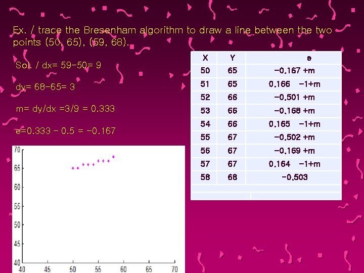
Ex. / trace the Bresenham algorithm to draw a line between the two points (50, 65), (59, 68). Sol. / dx= 59 -50= 9 dy= 68 -65= 3 m= dy/dx =3/9 = 0. 333 e=0. 333 – 0. 5 = -0. 167 X Y e 50 65 51 65 52 66 -0. 501 +m 53 66 -0. 168 +m 54 66 55 67 -0. 502 +m 56 67 -0. 169 +m 57 67 58 68 -0. 167 +m 0. 166 0. 165 0. 164 -1+m -0. 503

Thank you