Computer Graphics Chapter 2 First Lecture TwoDimensional Graphics

Computer Graphics Chapter 2 First Lecture

Two-Dimensional Graphics

Introduction • In order to draw a picture on a raster display, we must determine the corresponding points in the frame buffer that make up the picture. To perform this task we must write scan conversion point plotting algorithms. • Both the frame buffer and the display screen are given a two-dimensional coordinates system with the origin at the lower left corner.

2. 1 Pixels, Coordinates, and Colors • To create a two-dimensional image, each point in the image is assigned a color. A point in 2 D can be identified by a pair of numerical coordinates. Colors can also be specified numerically. However, the assignment of numbers to points or colors is somewhat arbitrary. • So we need to spend some time studying coordinate systems, which associate numbers to points, and color models, which associate numbers to colors.

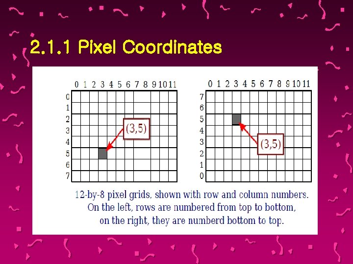
2. 1. 1 Pixel Coordinates • A digital image is made up of rows and columns of pixels. A pixel in such an image can be specified by saying which column and which row contains it. In terms of coordinates, a pixel can be identified by a pair of integers giving the column number and the row number. For example, the pixel with coordinates (3, 5) would lie in column number 3 and row number 5.

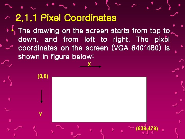
2. 1. 1 Pixel Coordinates • Conventionally, columns are numbered from left to right, starting with zero. Most graphics systems, including the ones we will study in this chapter, number rows from top to bottom, starting from zero.

2. 1. 1 Pixel Coordinates

2. 1. 1 Pixel Coordinates • To draw a point on the Matlab panel, a point plotting procedure is required. We assume the availability of the command: plot (x , y , color)

2. 1. 1 Pixel Coordinates • The drawing on the screen starts from top to down, and from left to right. The pixel coordinates on the screen (VGA 640´ 480) is shown in figure below: X (0, 0) Y (639, 479)

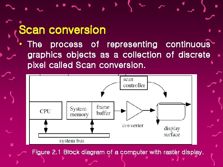
Scan conversion • The process of representing continuous graphics objects as a collection of discrete pixel called Scan conversion. Figure 2. 1 Block diagram of a computer with raster display.

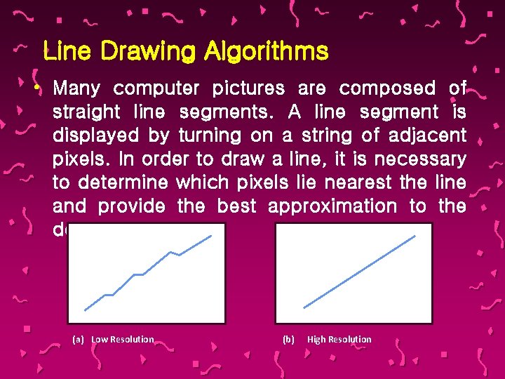
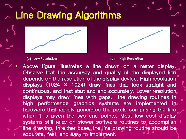
Line Drawing Algorithms • Many computer pictures are composed of straight line segments. A line segment is displayed by turning on a string of adjacent pixels. In order to draw a line, it is necessary to determine which pixels lie nearest the line and provide the best approximation to the desired line. (a) Low Resolution (b) High Resolution

Line Drawing Algorithms (a) Low Resolution (b) High Resolution • Above figure illustrates a line drawn on a raster display. Observe that the accuracy and quality of the displayed line depends on the resolution of the display device. High resolution displays (1024 × 1024) draw lines that look straight and continuous, and that start and end accurately. Lower resolution displays may draw lines with gaps. Line drawing routines in high performance graphics systems are implemented in hardware that rapidly generates the pixels comprising the line when it is given the two end points. Most low cost display systems still relay on slower software routines to accomplish line drawing. In either case, the line drawing routine should be accurate, fast, and easy to implement.

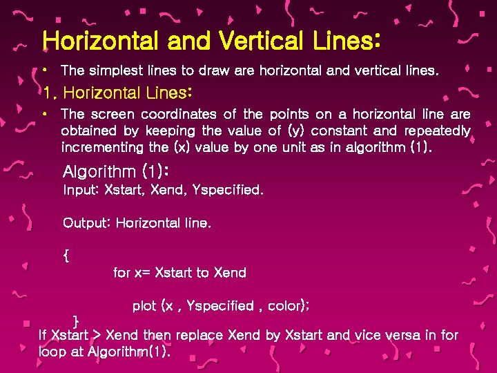
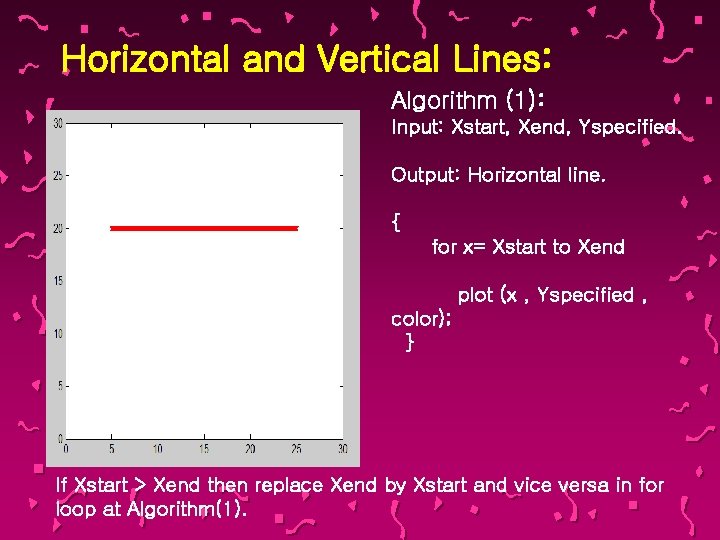
Horizontal and Vertical Lines: • The simplest lines to draw are horizontal and vertical lines. 1. Horizontal Lines: • The screen coordinates of the points on a horizontal line are obtained by keeping the value of (y) constant and repeatedly incrementing the (x) value by one unit as in algorithm (1). Algorithm (1): Input: Xstart, Xend, Yspecified. Output: Horizontal line. { for x= Xstart to Xend plot (x , Yspecified , color); } If Xstart > Xend then replace Xend by Xstart and vice versa in for loop at Algorithm(1).

Horizontal and Vertical Lines: Algorithm (1): Input: Xstart, Xend, Yspecified. Output: Horizontal line. { for x= Xstart to Xend plot (x , Yspecified , color); } If Xstart > Xend then replace Xend by Xstart and vice versa in for loop at Algorithm(1).

Horizontal and Vertical Lines: 2. Vertical Lines: • The screen coordinates of the points on a vertical line are obtained by keeping the value of (x) constant and repeatedly incrementing the (y) value by one unit as in algorithm (2). Algorithm (2): Input: Ystart, Yend, Xspecified. Output: Vertical line. { for y= Ystart to Yend plot (Xspecified , y , color); } If Ystart > Yend then replace Yend by Ystart and vice versa in for loop at algorithm (2).

Horizontal and Vertical Lines: Algorithm (2): Input: Ystart, Yend, Xspecified Output: Vertical line. { for y= Ystart to Yend plot (Xspecified , y , color); } If Ystart > Yend then replace Yend by Ystart and vice versa in for loop at algorithm (2).

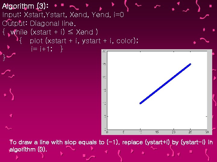
Horizontal and Vertical Lines: 3. Diagonal Lines: • To draw a diagonal line with a slope equal to (+1), we need only repeatedly increment by one unit both x and y values from the start to end pixels as shown in algorithm (3). Algorithm (3): Input: Xstart, Ystart, Xend, Yend. i=0 Output: Diagonal line. { while (xstart + i) ≤ Xend ) { plot (xstart + i, ystart + i, color); i= i+1; } } To draw a line with slop equals to (-1), replace (ystart+i) by (ystart-i) in algorithm (3).

Algorithm (3): Input: Xstart, Ystart, Xend, Yend. i=0 Output: Diagonal line. { while (xstart + i) ≤ Xend ) { plot (xstart + i, ystart + i, color); i= i+1; } } To draw a line with slop equals to (-1), replace (ystart+i) by (ystart-i) in algorithm (3).

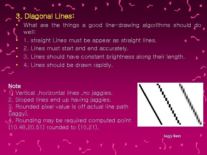
3. Diagonal Lines: • What are things a good line-drawing algorithms should do well: • 1. straight Lines must be appear as straight lines. • 2. Lines must start and end accurately. • 3. Lines should have constant brightness along their length. • 4. Lines should be drawn rapidly. Note 1. Vertical , horizontal lines , no jaggies. 2. Sloped lines end up having jaggies. 3. Rounded pixel value is off actual line path (jaggy). 4. Rounding may be required computed point (10. 48, 20. 51) rounded to (10, 21). Jaggy lines