Computer Aided Geometric Design Introduction Milind Sohoni Department

Computer Aided Geometric Design Introduction Milind Sohoni Department of Computer Science and Engg. IIT Powai Email: sohoni@cse. iitb. ac. in Sources: www. cse. iitb. ac. in/sohoni/gsslcourse

A Solid Modeling Fable • • Ahmedabad-Visual Design Office Kolhapur-Mechanical Design Office Saki Naka – Die Manufacturer Lucknow- Soap manufacturer

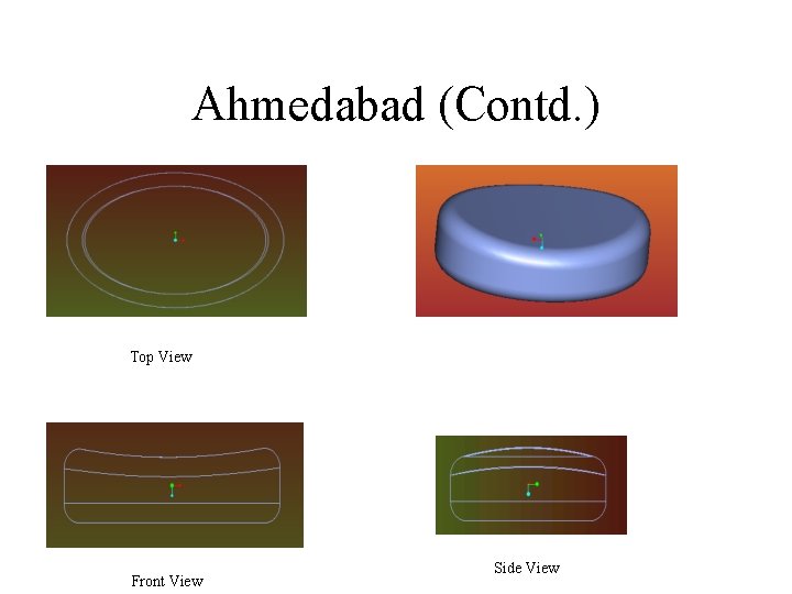
Ahmedabad-Visual Design • Input: A dream soap tablet • Output: • Sketches/Drawings • Weights • Packaging needs

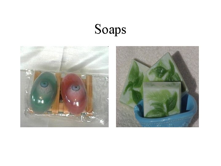
Soaps

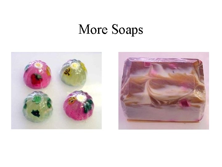
More Soaps

Ahmedabad (Contd. ) Top View Front View Side View

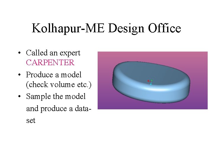
Kolhapur-ME Design Office • Called an expert CARPENTER • Produce a model (check volume etc. ) • Sample the model and produce a dataset

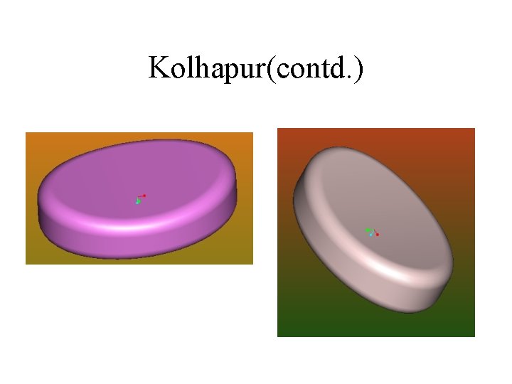
Kolhapur(contd. )

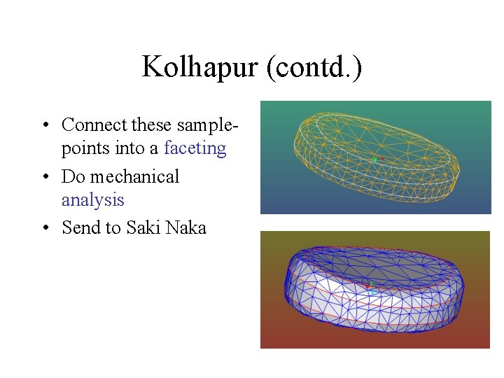
Kolhapur (contd. ) • Connect these samplepoints into a faceting • Do mechanical analysis • Send to Saki Naka

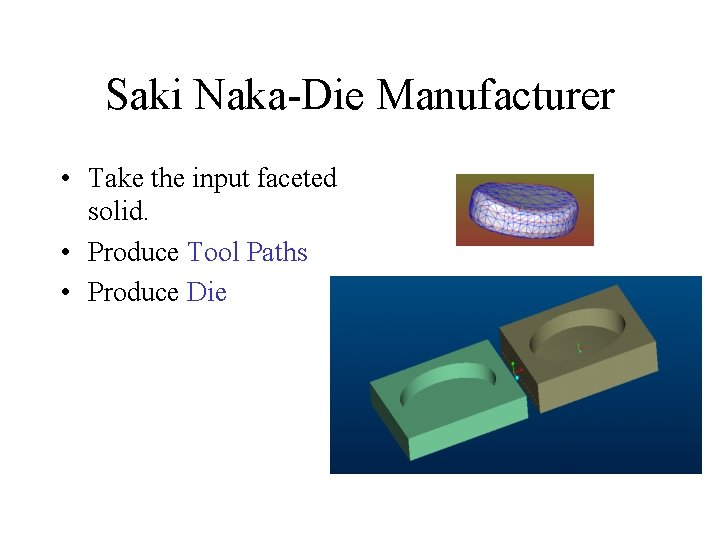
Saki Naka-Die Manufacturer • Take the input faceted solid. • Produce Tool Paths • Produce Die

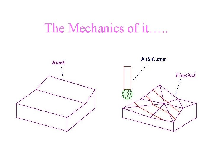
The Mechanics of it…. .

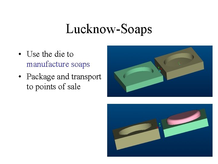
Lucknow-Soaps • Use the die to manufacture soaps • Package and transport to points of sale

Problems began… • • The die degraded in Lucknow The Carpenter died in Kolhapur Saki Naka upgraded its CNC machine The wooden model eroded But The Drawings were there!

So Then…. • The same process was repeated but… The shape was different! The customer was suspicious and sales dropped!!!

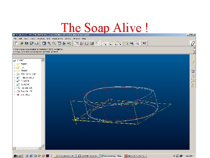
The Soap Alive !

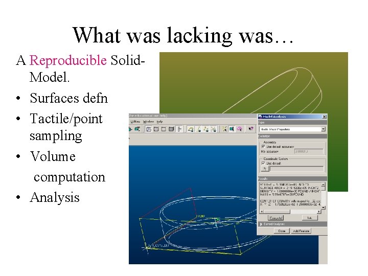
What was lacking was… A Reproducible Solid. Model. • Surfaces defn • Tactile/point sampling • Volume computation • Analysis

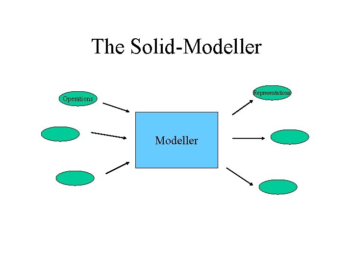
The Solid-Modeller Representations Operations Modeller

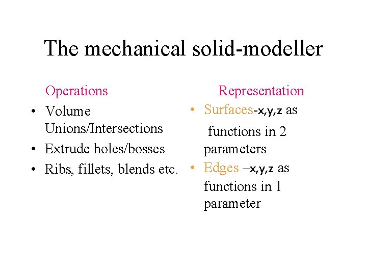
The mechanical solid-modeller Operations Representation • Surfaces-x, y, z as • Volume Unions/Intersections functions in 2 • Extrude holes/bosses parameters • Ribs, fillets, blends etc. • Edges –x, y, z as functions in 1 parameter

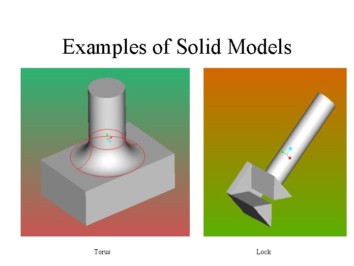
Examples of Solid Models Torus Lock

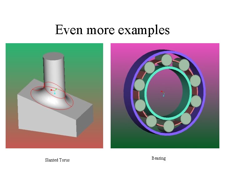
Even more examples Slanted Torus Bearing

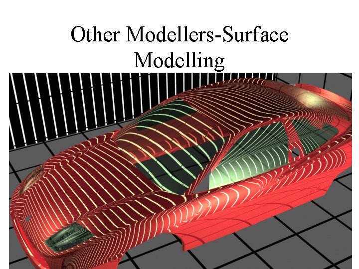
Other Modellers-Surface Modelling

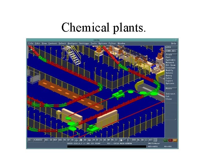
Chemical plants.

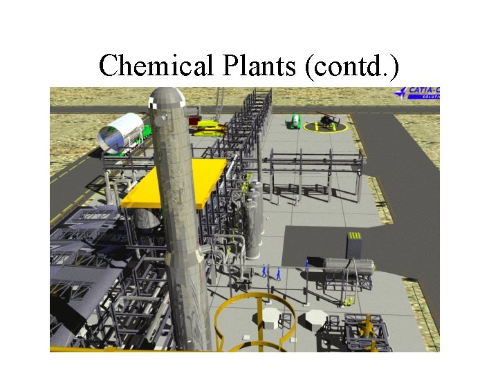
Chemical Plants (contd. )

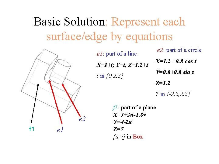
Basic Solution: Represent each surface/edge by equations e 2: part of a circle e 1: part of a line X=1+t; Y=t, Z=1. 2+t t in [0, 2. 3] X=1. 2 +0. 8 cos t Y=0. 8+0. 8 sin t Z=1. 2 T in [-2. 3, 2. 3] e 2 f 1 e 1 f 1: part of a plane X=3+2 u-1. 8 v Y=4 -2 u Z=7 [u, v] in Box

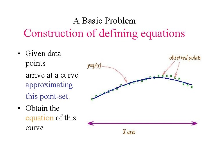
A Basic Problem Construction of defining equations • Given data points arrive at a curve approximating this point-set. • Obtain the equation of this curve

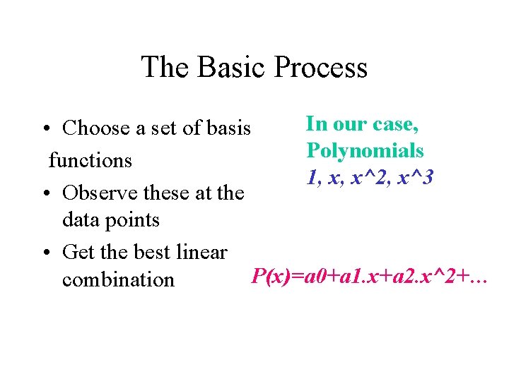
The Basic Process In our case, • Choose a set of basis Polynomials functions 1, x, x^2, x^3 • Observe these at the data points • Get the best linear P(x)=a 0+a 1. x+a 2. x^2+… combination

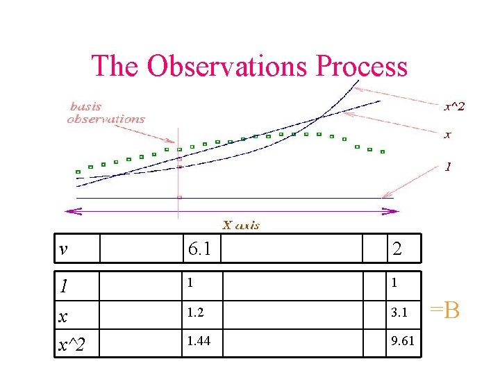
The Observations Process v 6. 1 2 1 1 1 x x^2 1. 2 3. 1 1. 44 9. 61 =B

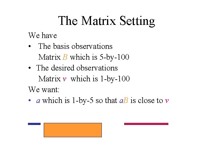
The Matrix Setting We have • The basis observations Matrix B which is 5 -by-100 • The desired observations Matrix v which is 1 -by-100 We want: • a which is 1 -by-5 so that a. B is close to v

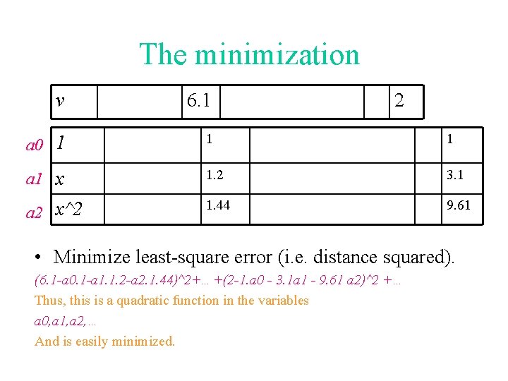
The minimization v 6. 1 2 a 0 1 1 1 a 1 x 1. 2 3. 1 a 2 x^2 1. 44 9. 61 • Minimize least-square error (i. e. distance squared). (6. 1 -a 0. 1 -a 1. 1. 2 -a 2. 1. 44)^2+…+(2 -1. a 0 - 3. 1 a 1 - 9. 61 a 2)^2 +… Thus, this is a quadratic function in the variables a 0, a 1, a 2, … And is easily minimized.

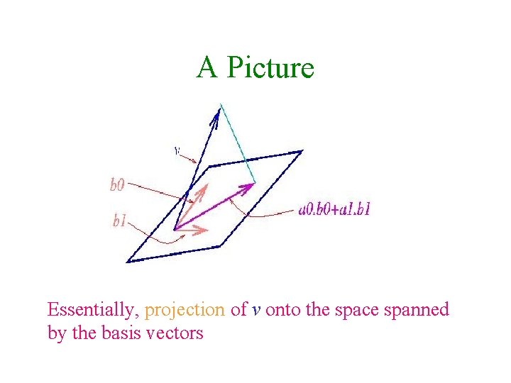
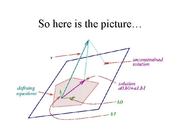
A Picture Essentially, projection of v onto the space spanned by the basis vectors

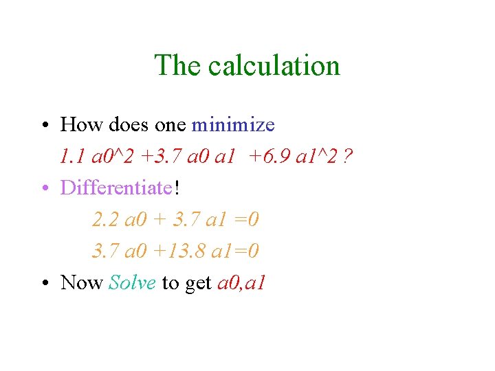
The calculation • How does one minimize 1. 1 a 0^2 +3. 7 a 0 a 1 +6. 9 a 1^2 ? • Differentiate! 2. 2 a 0 + 3. 7 a 1 =0 3. 7 a 0 +13. 8 a 1=0 • Now Solve to get a 0, a 1

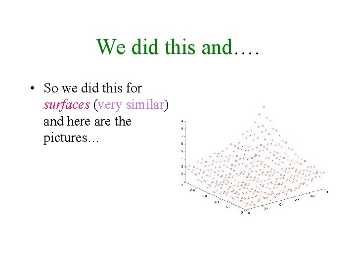
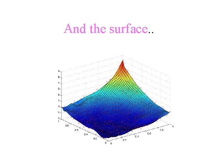
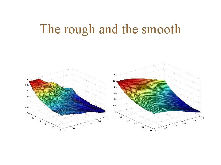
We did this and…. • So we did this for surfaces (very similar) and here are the pictures…

And the surface. .

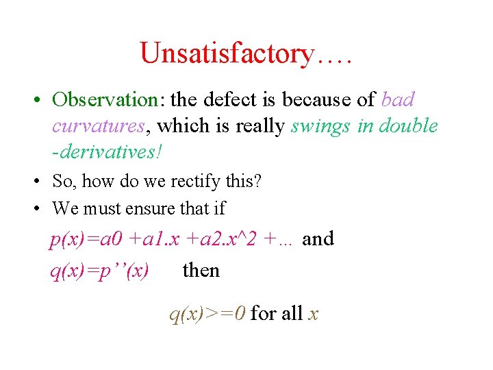
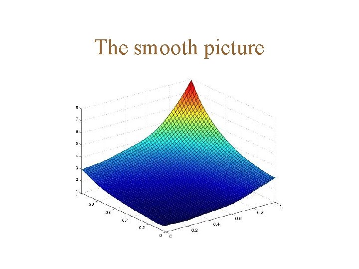
Unsatisfactory…. • Observation: the defect is because of bad curvatures, which is really swings in double -derivatives! • So, how do we rectify this? • We must ensure that if p(x)=a 0 +a 1. x +a 2. x^2 +… and q(x)=p’’(x) then q(x)>=0 for all x

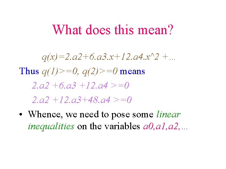
What does this mean? q(x)=2. a 2+6. a 3. x+12. a 4. x^2 +… Thus q(1)>=0, q(2)>=0 means 2. a 2 +6. a 3 +12. a 4 >=0 2. a 2 +12. a 3+48. a 4 >=0 • Whence, we need to pose some linear inequalities on the variables a 0, a 1, a 2, …

So here is the picture…

The smooth picture

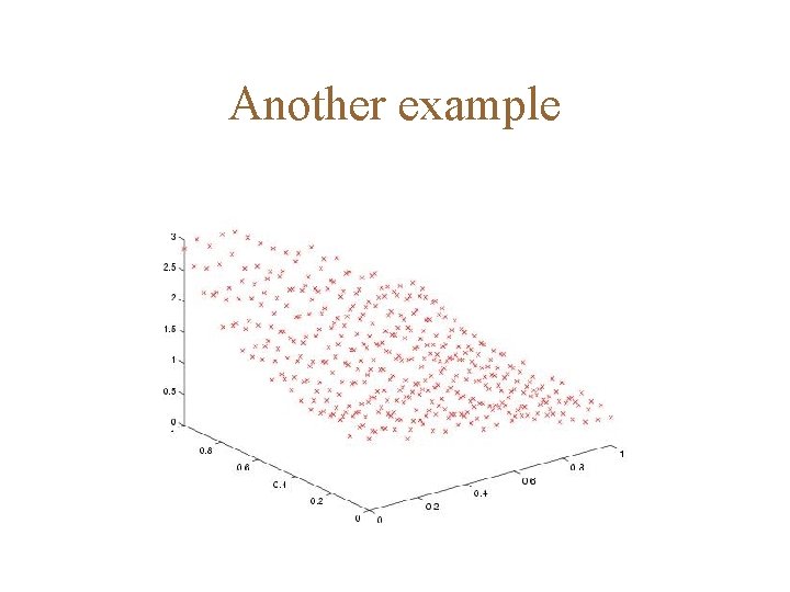
Another example

The rough and the smooth

Summary • • The Solid Modeler Boundary Representation Polynomials and Splines Operations Optimization Curvatures and Basic differential geometry Genus MATLAB Softwares Pro. Engineer