Computational Vision Edge Detection Canny Detector Line Detection

Computational Vision § Edge Detection § Canny Detector § Line Detection § Hough Transform § Trucco: Chapter 4, pp. 76 – 80 Chapter 5, pp. 95 - 100 Computational Vision / Ioannis Stamos

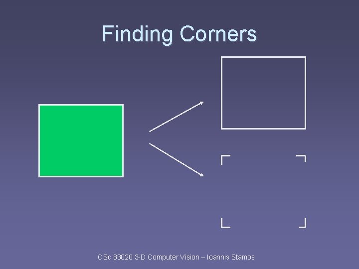
Finding Corners CSc 83020 3 -D Computer Vision – Ioannis Stamos

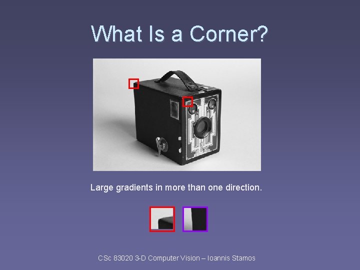
What Is a Corner? Large gradients in more than one direction. CSc 83020 3 -D Computer Vision – Ioannis Stamos

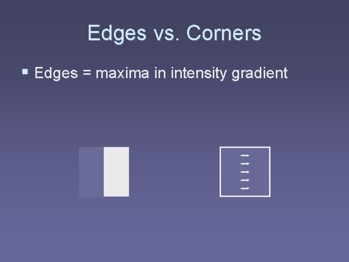
Edges vs. Corners § Edges = maxima in intensity gradient

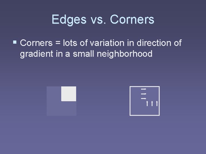
Edges vs. Corners § Corners = lots of variation in direction of gradient in a small neighborhood

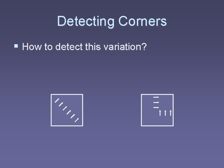
Detecting Corners § How to detect this variation?

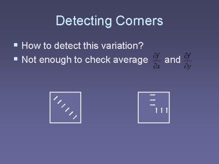
Detecting Corners § How to detect this variation? § Not enough to check average and

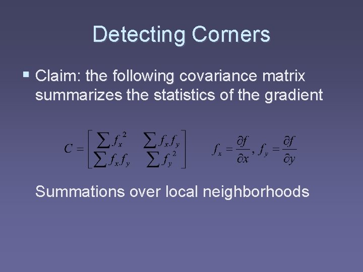
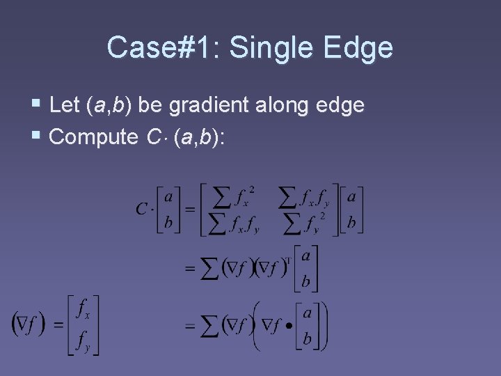
Detecting Corners § Claim: the following covariance matrix summarizes the statistics of the gradient Summations over local neighborhoods

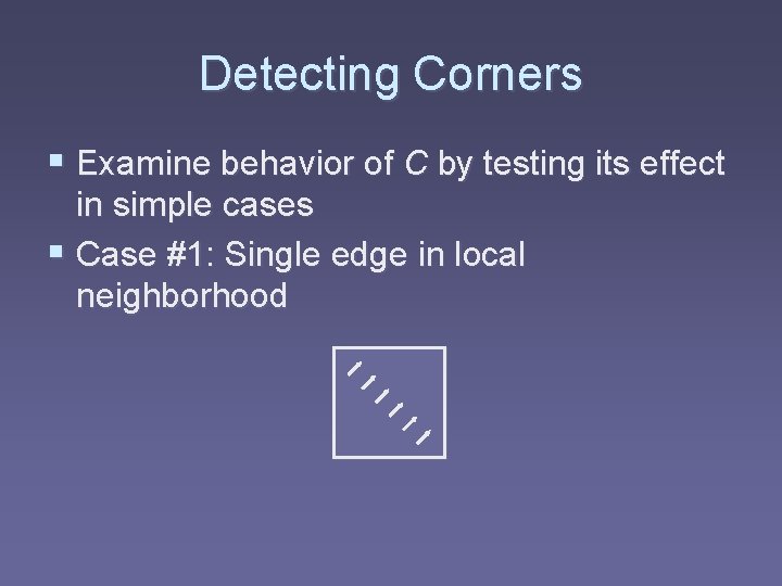
Detecting Corners § Examine behavior of C by testing its effect in simple cases § Case #1: Single edge in local neighborhood

Case#1: Single Edge § Let (a, b) be gradient along edge § Compute C (a, b):

Case #1: Single Edge § However, in this simple case, the only nonzero terms are those where f = (a, b) § So, C (a, b) is just some multiple of (a, b)

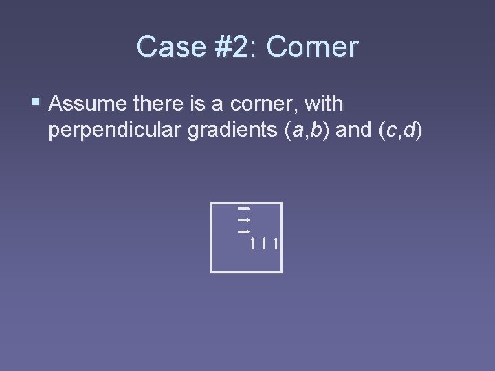
Case #2: Corner § Assume there is a corner, with perpendicular gradients (a, b) and (c, d)

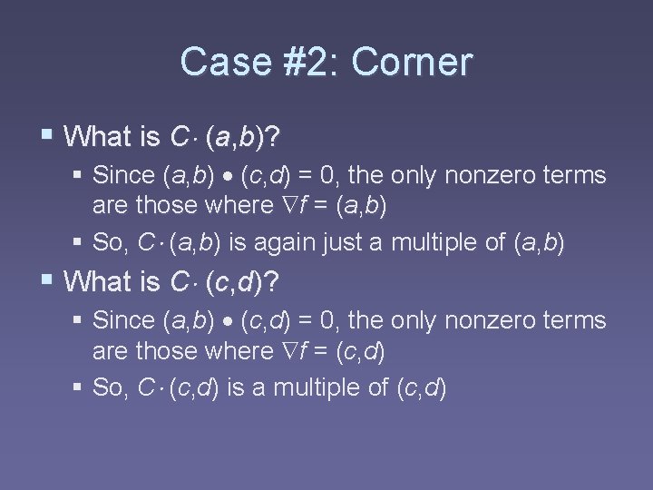
Case #2: Corner § What is C (a, b)? § Since (a, b) (c, d) = 0, the only nonzero terms are those where f = (a, b) § So, C (a, b) is again just a multiple of (a, b) § What is C (c, d)? § Since (a, b) (c, d) = 0, the only nonzero terms are those where f = (c, d) § So, C (c, d) is a multiple of (c, d)

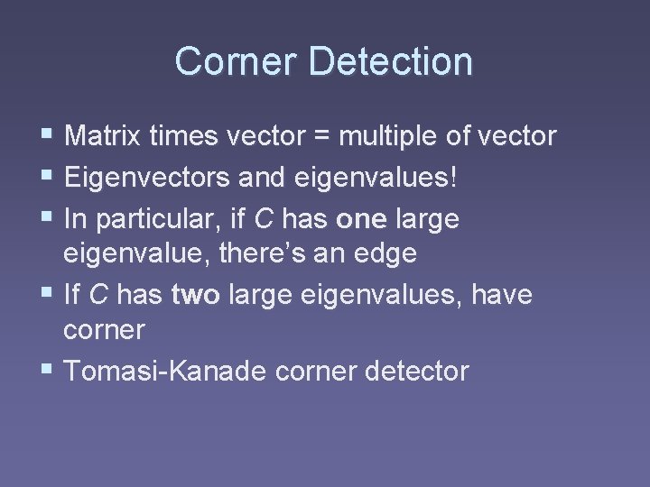
Corner Detection § Matrix times vector = multiple of vector § Eigenvectors and eigenvalues! § In particular, if C has one large eigenvalue, there’s an edge § If C has two large eigenvalues, have corner § Tomasi-Kanade corner detector

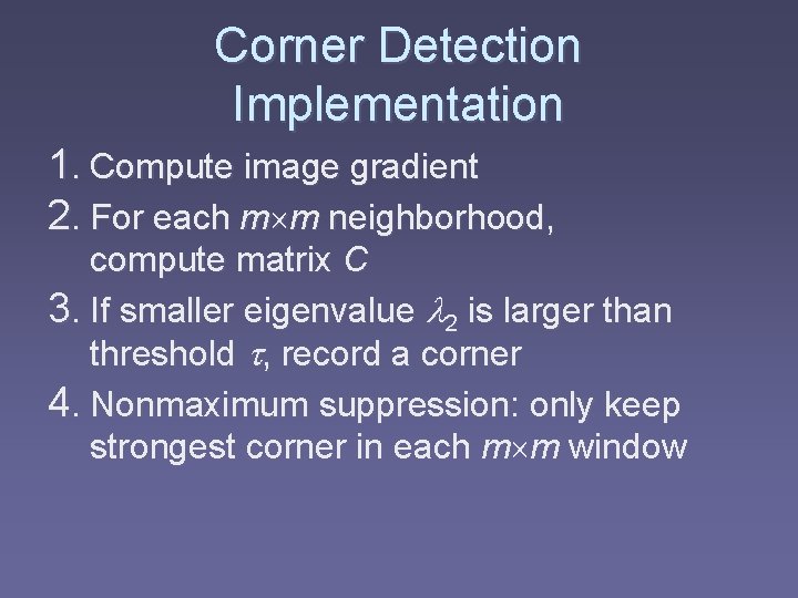
Corner Detection Implementation 1. Compute image gradient 2. For each m m neighborhood, compute matrix C 3. If smaller eigenvalue 2 is larger than threshold , record a corner 4. Nonmaximum suppression: only keep strongest corner in each m m window

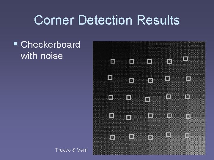
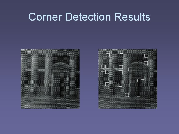
Corner Detection Results § Checkerboard with noise Trucco & Verri

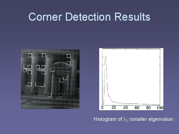
Corner Detection Results

Corner Detection Results Histogram of l 2 (smaller eigenvalue)

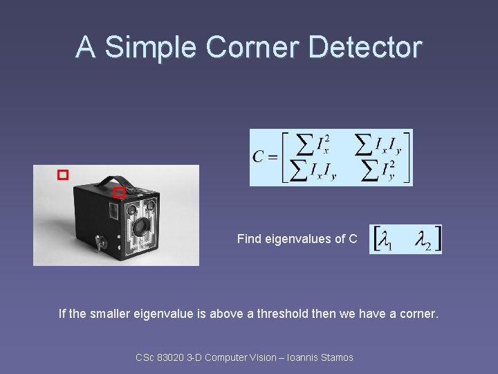
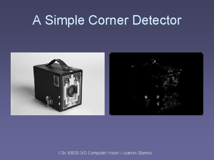
A Simple Corner Detector Find eigenvalues of C If the smaller eigenvalue is above a threshold then we have a corner. CSc 83020 3 -D Computer Vision – Ioannis Stamos

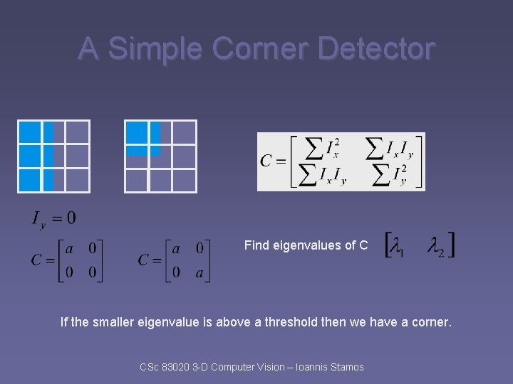
A Simple Corner Detector Find eigenvalues of C If the smaller eigenvalue is above a threshold then we have a corner. CSc 83020 3 -D Computer Vision – Ioannis Stamos

A Simple Corner Detector CSc 83020 3 -D Computer Vision – Ioannis Stamos

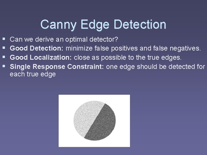
Canny Edge Detection § § Can we derive an optimal detector? Good Detection: minimize false positives and false negatives. Good Localization: close as possible to the true edges. Single Response Constraint: one edge should be detected for each true edge

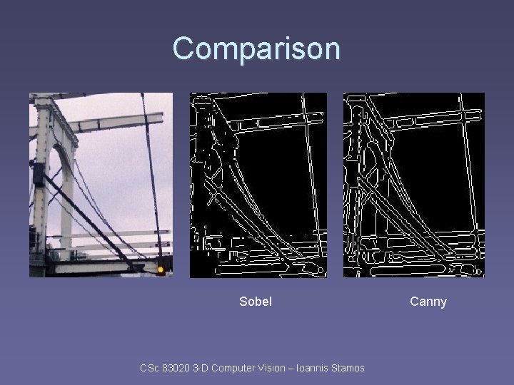
Comparison Sobel CSc 83020 3 -D Computer Vision – Ioannis Stamos Canny

Canny Edge Detection § 3 STEPS: § CANNY_ENHANCER § NONMAX_SUPPRESION § HYSTERESIS_THRESH

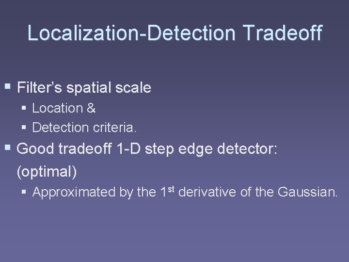
Localization-Detection Tradeoff § Filter’s spatial scale § Location & § Detection criteria. § Good tradeoff 1 -D step edge detector: (optimal) § Approximated by the 1 st derivative of the Gaussian.

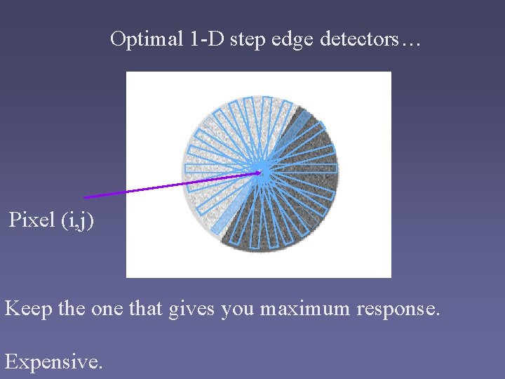
Optimal 1 -D step edge detectors… Pixel (i, j) Keep the one that gives you maximum response. Expensive.

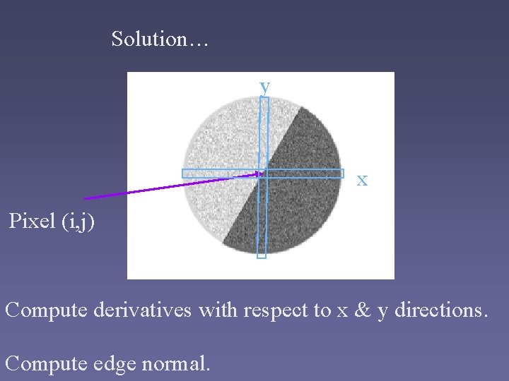
Solution… y x Pixel (i, j) Compute derivatives with respect to x & y directions. Compute edge normal.

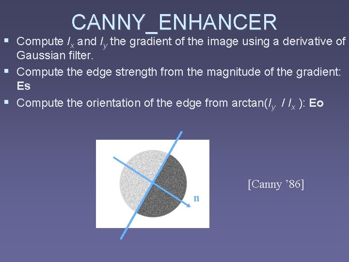
CANNY_ENHANCER § Compute Ix and Iy the gradient of the image using a derivative of Gaussian filter. § Compute the edge strength from the magnitude of the gradient: Es § Compute the orientation of the edge from arctan(Iy / Ix ): Eo [Canny ’ 86] n

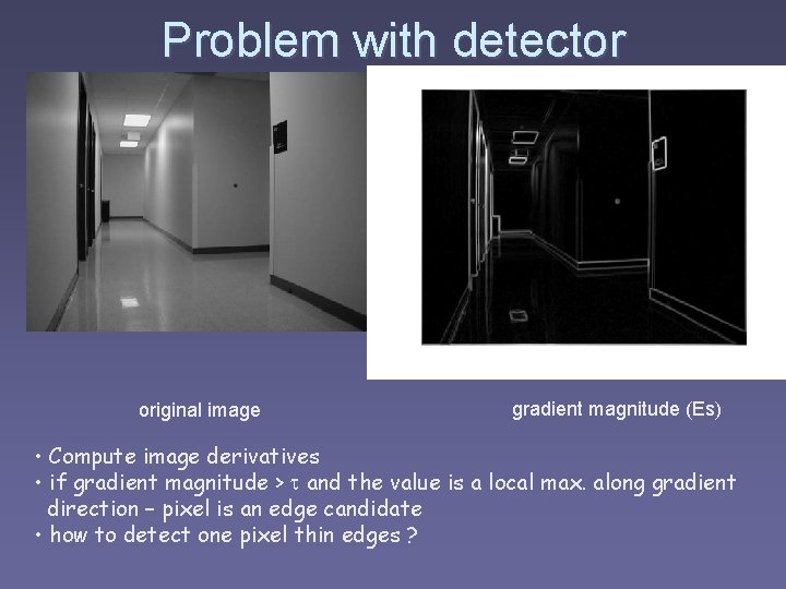
Problem with detector original image gradient magnitude (Es) • Compute image derivatives • if gradient magnitude > and the value is a local max. along gradient direction – pixel is an edge candidate • how to detect one pixel thin edges ?

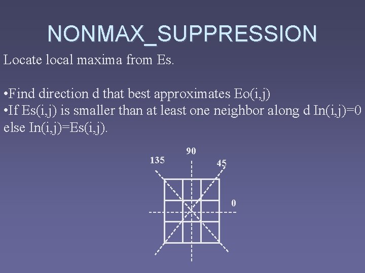
NONMAX_SUPPRESSION Locate local maxima from Es. • Find direction d that best approximates Eo(i, j) • If Es(i, j) is smaller than at least one neighbor along d In(i, j)=0 else In(i, j)=Es(i, j). 135 90 45 0

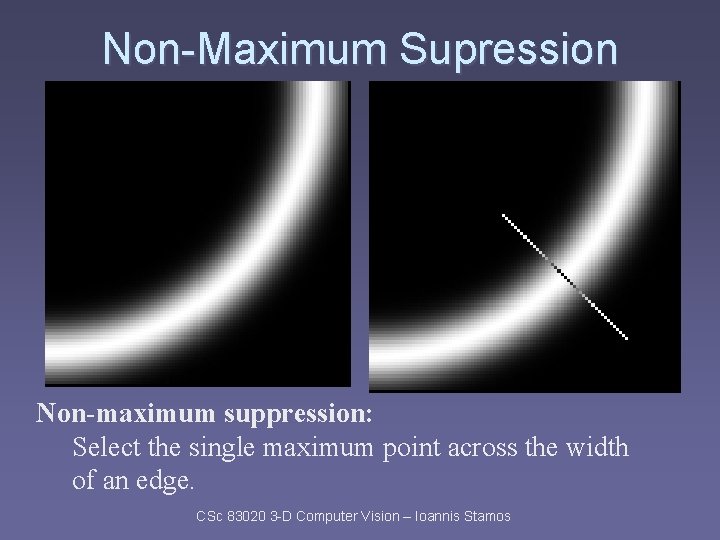
Non-Maximum Supression Non-maximum suppression: Select the single maximum point across the width of an edge. CSc 83020 3 -D Computer Vision – Ioannis Stamos

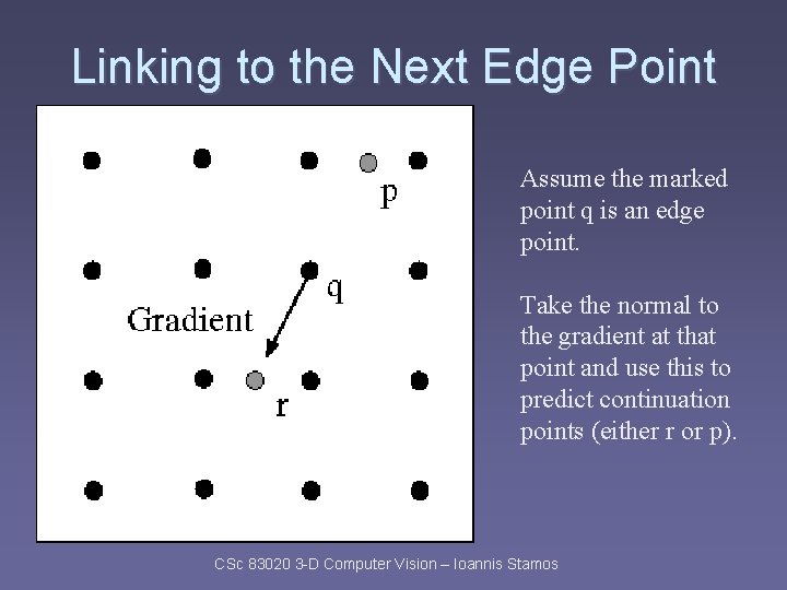
Linking to the Next Edge Point Assume the marked point q is an edge point. Take the normal to the gradient at that point and use this to predict continuation points (either r or p). CSc 83020 3 -D Computer Vision – Ioannis Stamos

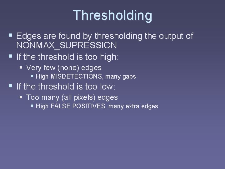
Thresholding § Edges are found by thresholding the output of NONMAX_SUPRESSION § If the threshold is too high: § Very few (none) edges § High MISDETECTIONS, many gaps § If the threshold is too low: § Too many (all pixels) edges § High FALSE POSITIVES, many extra edges

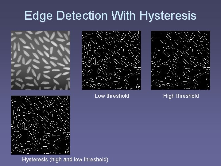
Edge Detection With Hysteresis Low threshold Hysteresis (high and low threshold) High threshold

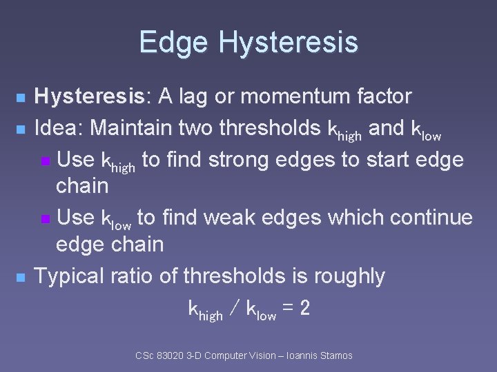
Edge Hysteresis n n n Hysteresis: A lag or momentum factor Idea: Maintain two thresholds khigh and klow n Use khigh to find strong edges to start edge chain n Use klow to find weak edges which continue edge chain Typical ratio of thresholds is roughly khigh / klow = 2 CSc 83020 3 -D Computer Vision – Ioannis Stamos

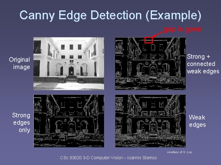
Edge Tracking Hysteresis thresholding [Canny ’ 86] Weak edges Strong edges reinforce weak edges Weak edge removed We call a pixel an edge if it is strong. We also call a pixel an edge if it is weak but is connected to an edge. A pixel is connected to an edge if it is in a direction perpendicular to the edge normal

Canny Edge Detection (Example) gap is gone Strong + connected weak edges Original image Strong edges only Weak edges courtesy of G. Loy CSc 83020 3 -D Computer Vision – Ioannis Stamos

HYSTERESIS_THRESH § Input: In, Eo, high threshold, low threshold. § Output: Lists of connected edges (contours).

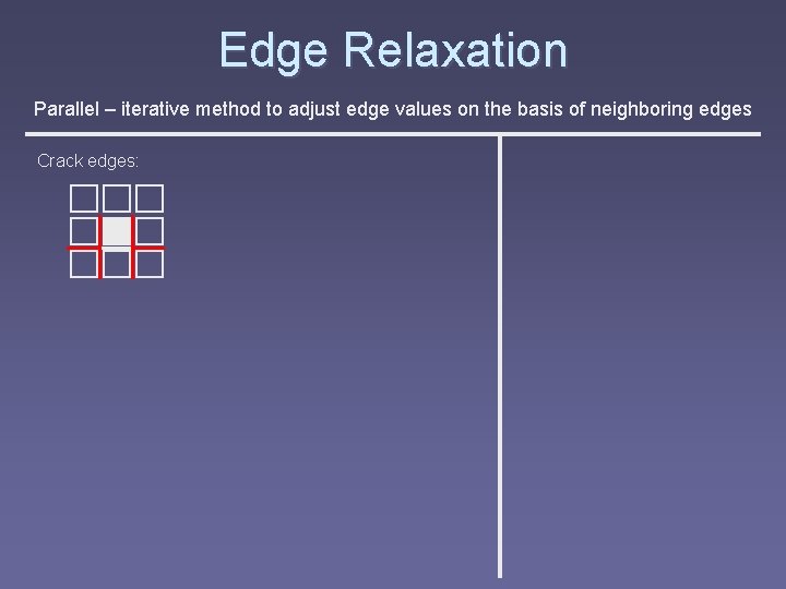
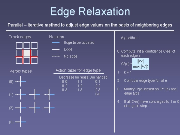
Edge Relaxation Parallel – iterative method to adjust edge values on the basis of neighboring edges Crack edges:

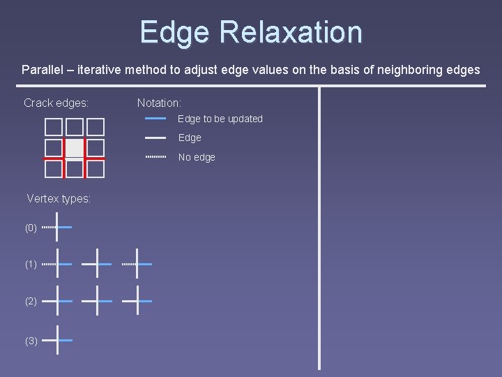
Edge Relaxation Parallel – iterative method to adjust edge values on the basis of neighboring edges Crack edges: Notation: Edge to be updated Edge No edge Vertex types: (0) (1) (2) (3)

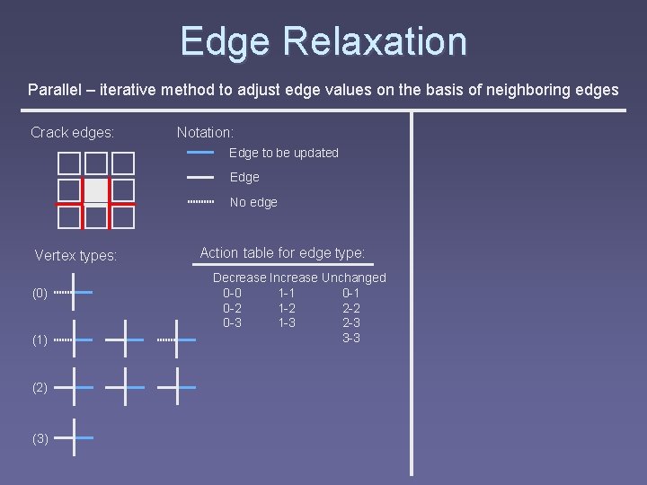
Edge Relaxation Parallel – iterative method to adjust edge values on the basis of neighboring edges Crack edges: Notation: Edge to be updated Edge No edge Vertex types: (0) (1) (2) (3) Action table for edge type: Decrease Increase Unchanged 0 -0 1 -1 0 -2 1 -2 2 -2 0 -3 1 -3 2 -3 3 -3

Edge Relaxation Parallel – iterative method to adjust edge values on the basis of neighboring edges Crack edges: Notation: Algorithm: Edge to be updated Edge No edge 0. Compute initial confidence C 0(e) of each edge e C 0(e) = Vertex types: (0) (1) (2) (3) Action table for edge type: Decrease Increase Unchanged 0 -0 1 -1 0 -2 1 -2 2 -2 0 -3 1 -3 2 -3 3 -3 1. k=1 2. Compute edge type for all e 3. Modify Ck(e) based on Ck-1(e) and edge type. 4. If all Ck(e) have converged to 1 or 0 else go to step 1

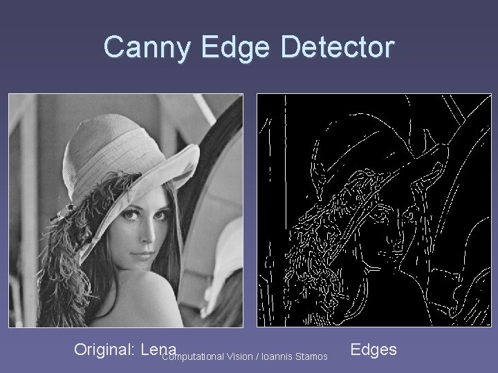
Canny Edge Detector Original: Lena Computational Vision / Ioannis Stamos Edges

Towards Global Features Local versus global CSc 83020 3 -D Computer Vision – Ioannis Stamos

From Edges to Lines CSc 83020 3 -D Computer Vision – Ioannis Stamos

Detecting Lines § What is the difference between line detection and edge detection? § Edges = local § Lines = nonlocal § Line detection usually performed on the output of an edge detector From Szymon Rusinkiewicz, Princeton

Detecting Lines § Possible approaches ? From Szymon Rusinkiewicz, Princeton

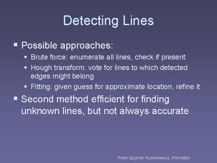
Detecting Lines § Possible approaches: § Brute force: enumerate all lines, check if present § Hough transform: vote for lines to which detected edges might belong § Fitting: given guess for approximate location, refine it § Second method efficient for finding unknown lines, but not always accurate From Szymon Rusinkiewicz, Princeton

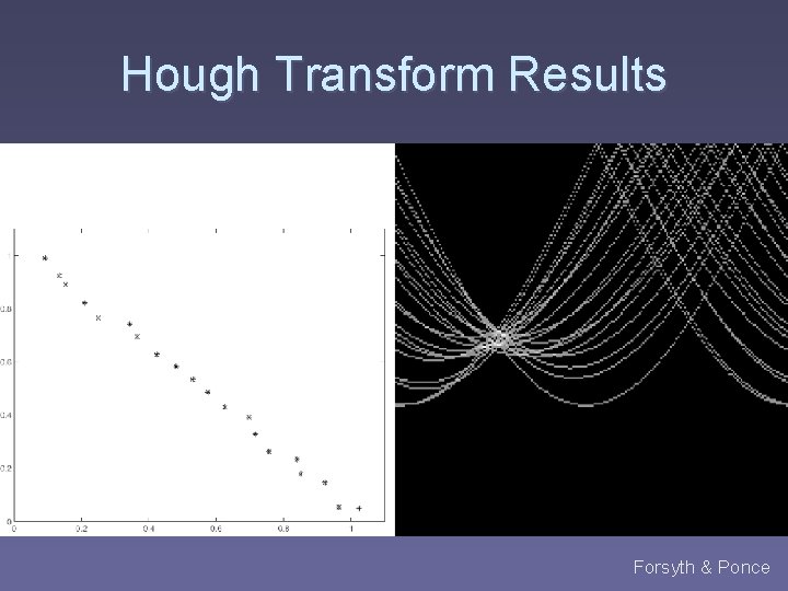
Hough Transform § General idea: transform from image coordinates to parameter space of feature § Need parameterized model of features § For each pixel, determine all parameter values that might have given rise to that pixel; vote § At end, look for peaks in parameter space From Szymon Rusinkiewicz, Princeton

Hough Transform for Lines § Generic line: y = ax+b § Parameters: a and b From Szymon Rusinkiewicz, Princeton

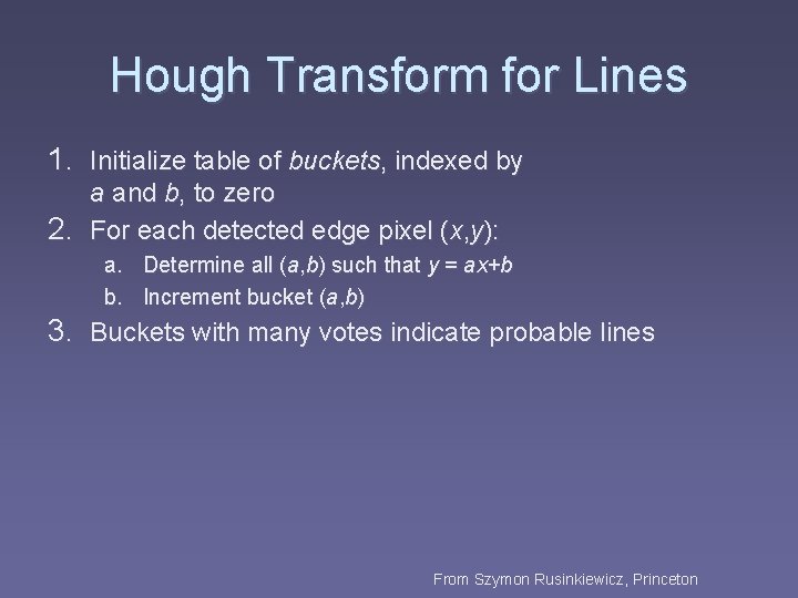
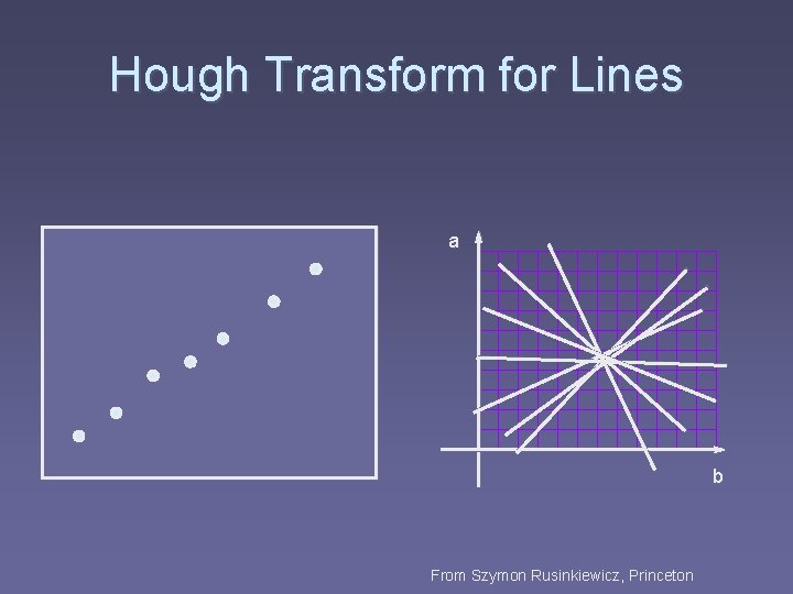
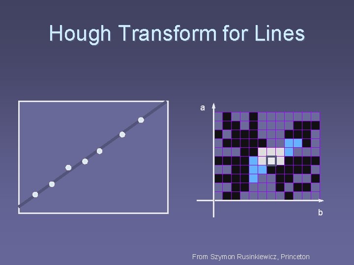
Hough Transform for Lines 1. Initialize table of buckets, indexed by a and b, to zero 2. For each detected edge pixel (x, y): a. Determine all (a, b) such that y = ax+b b. Increment bucket (a, b) 3. Buckets with many votes indicate probable lines From Szymon Rusinkiewicz, Princeton

Hough Transform for Lines a b From Szymon Rusinkiewicz, Princeton

Hough Transform for Lines a b From Szymon Rusinkiewicz, Princeton

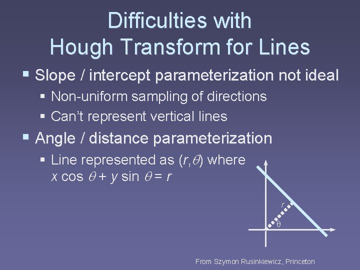
Difficulties with Hough Transform for Lines § Slope / intercept parameterization not ideal § Non-uniform sampling of directions § Can’t represent vertical lines § Angle / distance parameterization § Line represented as (r, q) where x cos q + y sin q = r r q From Szymon Rusinkiewicz, Princeton

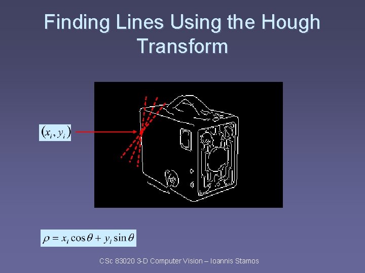
Finding Lines Using the Hough Transform CSc 83020 3 -D Computer Vision – Ioannis Stamos

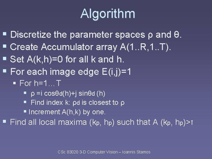
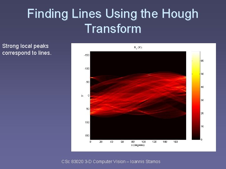
Algorithm § Discretize the parameter spaces ρ and θ. § Create Accumulator array A(1. . R, 1. . T). § Set A(k, h)=0 for all k and h. § For each image edge E(i, j)=1 § For h=1…T § ρ =i cosθd(h)+j sinθd (h) § Find index k: ρd is closest to ρ § Increment A(h, k) by one. § Find all local maxima (kp, hp) such that A (kp, hp)>τ CSc 83020 3 -D Computer Vision – Ioannis Stamos

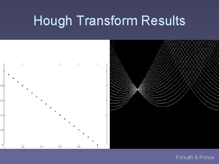
Hough Transform Results Forsyth & Ponce

Hough Transform Results Forsyth & Ponce

Finding Lines Using the Hough Transform Strong local peaks correspond to lines. CSc 83020 3 -D Computer Vision – Ioannis Stamos

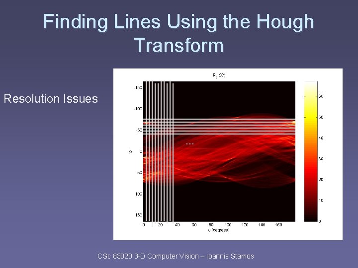
Finding Lines Using the Hough Transform Resolution Issues … CSc 83020 3 -D Computer Vision – Ioannis Stamos

Bucket Selection § How to select bucket size? From Szymon Rusinkiewicz, Princeton

Bucket Selection § How to select bucket size? § Too small: poor performance on noisy data, long running times § Too large: poor accuracy, possibility of false positives § Large buckets + verification and refinement § Problems distinguishing nearby lines § Be smarter at selecting buckets § Use gradient information to select subset of buckets § More sensitive to noise From Szymon Rusinkiewicz, Princeton

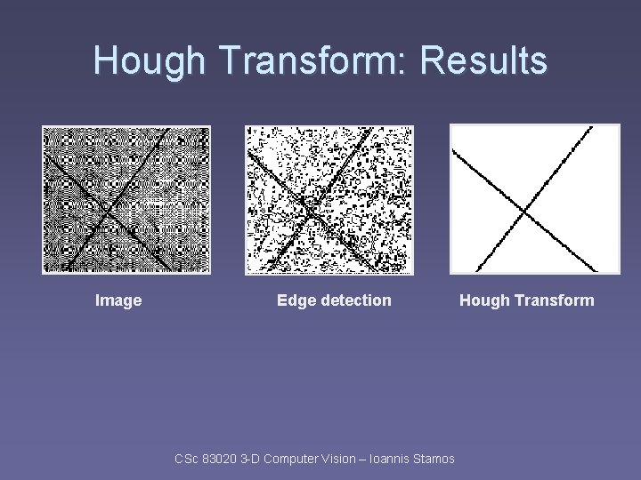
Hough Transform: Results Image Edge detection CSc 83020 3 -D Computer Vision – Ioannis Stamos Hough Transform

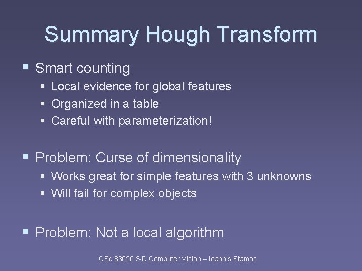
Summary Hough Transform § Smart counting § Local evidence for global features § Organized in a table § Careful with parameterization! § Problem: Curse of dimensionality § Works great for simple features with 3 unknowns § Will fail for complex objects § Problem: Not a local algorithm CSc 83020 3 -D Computer Vision – Ioannis Stamos

Hough Transform § What else can be detected using Hough transform?

Hough Transform § What else can be detected using Hough transform? § Anything, but dimensionality is key

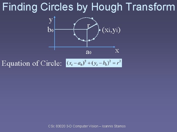
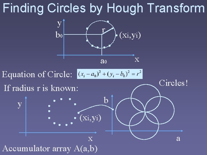
Finding Circles by Hough Transform y b 0 r a 0 (xi, yi) x Equation of Circle: CSc 83020 3 -D Computer Vision – Ioannis Stamos

Finding Circles by Hough Transform y b 0 r a 0 Equation of Circle: If radius r is known: (xi, yi) x Circles! b y (xi, yi) x Accumulator array A(a, b) a

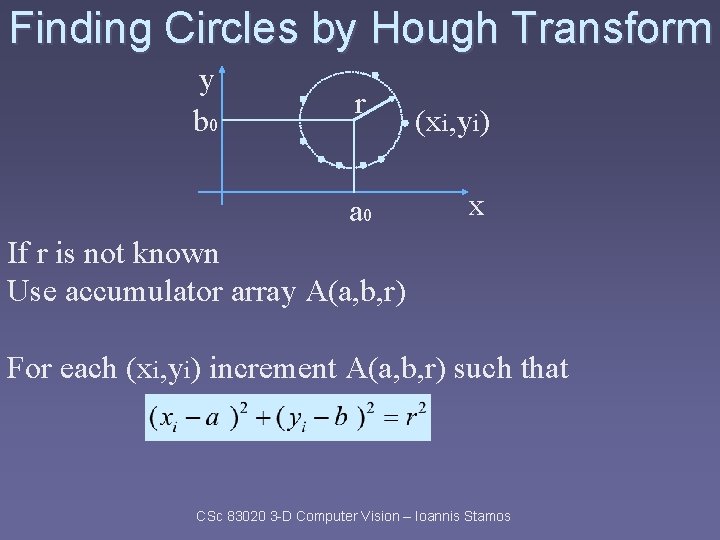
Finding Circles by Hough Transform y b 0 r a 0 (xi, yi) x If r is not known Use accumulator array A(a, b, r) For each (xi, yi) increment A(a, b, r) such that CSc 83020 3 -D Computer Vision – Ioannis Stamos

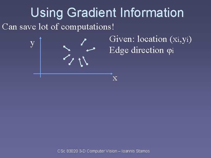
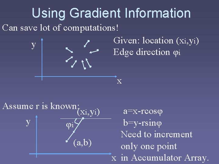
Using Gradient Information Can save lot of computations! Given: location (xi, yi) y Edge direction φi x CSc 83020 3 -D Computer Vision – Ioannis Stamos

Using Gradient Information Can save lot of computations! Given: location (xi, yi) y Edge direction φi x Assume r is known: (xi, yi) y φi (a, b) a=x-rcosφ b=y-rsinφ Need to increment only one point x in Accumulator Array.

Hough Transform for Curves § Curve y=f(x, a) § a=[a 1, … , ap] the parameters of the curve. § Limitation: size of parameter space wrt # of parameters. § Solution: variable-resolution parameter space. CSc 83020 3 -D Computer Vision – Ioannis Stamos

Hough Transform § Pattern Matching. § More efficient than template matching. § Handles occlusion. § Finds all instances of pattern. § Handling inaccurate edge locations? § Drawbacks?

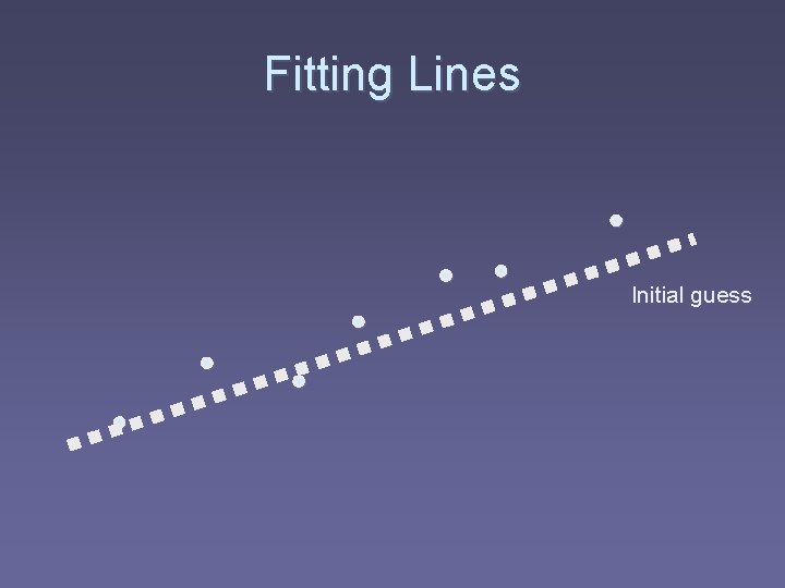
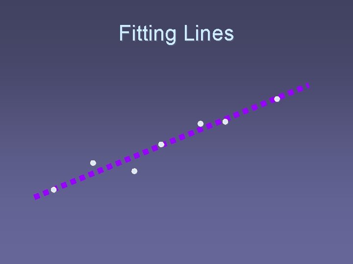
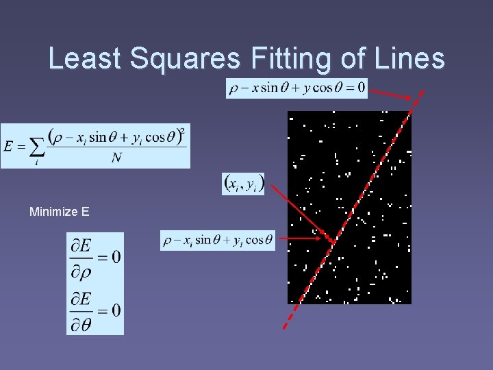
Fitting § Output of Hough transform often not accurate enough § Use as initial guess for fitting

Fitting Lines Initial guess

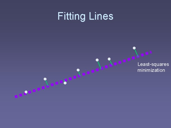
Fitting Lines Least-squares minimization

Fitting Lines

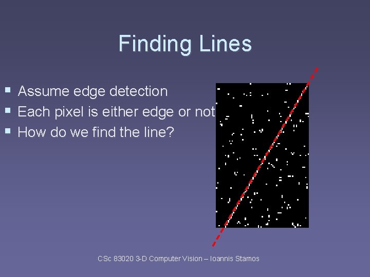
Finding Lines § § § Assume edge detection Each pixel is either edge or not How do we find the line? CSc 83020 3 -D Computer Vision – Ioannis Stamos

Finding Lines § § § Assume edge detection Each pixel is either edge or not How do we find the line? CSc 83020 3 -D Computer Vision – Ioannis Stamos

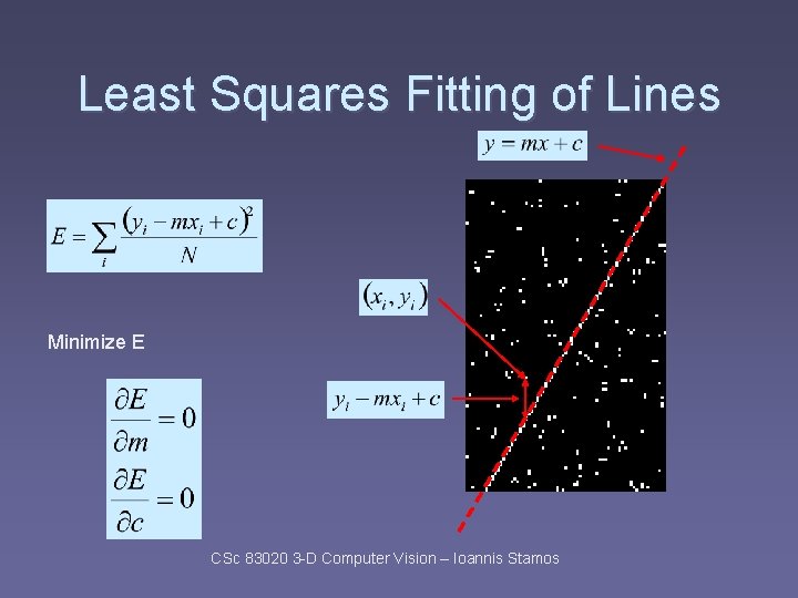
Least Squares Fitting of Lines Minimize E CSc 83020 3 -D Computer Vision – Ioannis Stamos

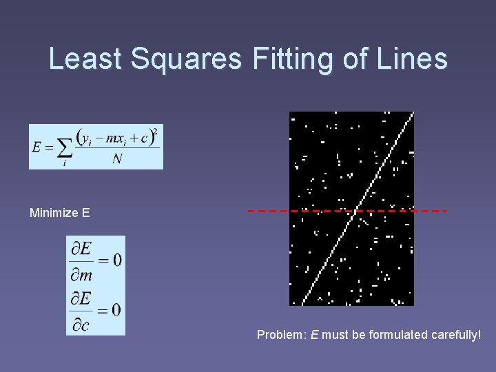
Least Squares Fitting of Lines Minimize E Problem: E must be formulated carefully!

Least Squares Fitting of Lines Minimize E