Computational Science Algorithms 1 Computational science Simulations of

Computational Science Algorithms 1

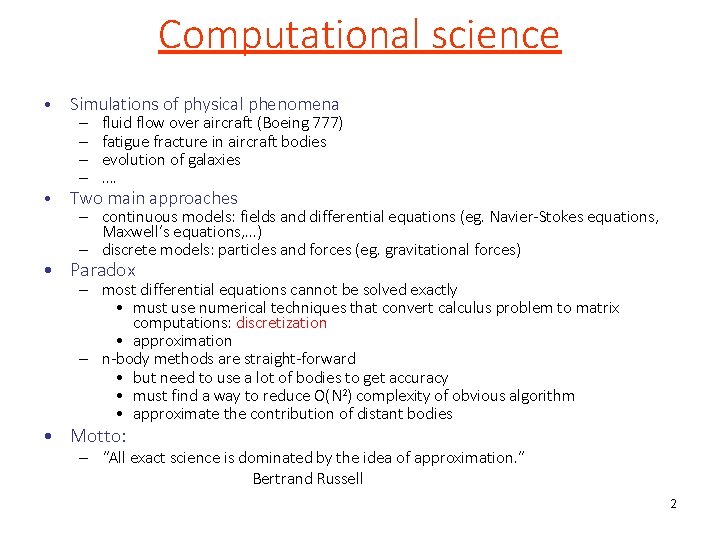
Computational science • Simulations of physical phenomena – – fluid flow over aircraft (Boeing 777) fatigue fracture in aircraft bodies evolution of galaxies …. • Two main approaches – continuous models: fields and differential equations (eg. Navier-Stokes equations, Maxwell’s equations, …) – discrete models: particles and forces (eg. gravitational forces) • Paradox – most differential equations cannot be solved exactly • must use numerical techniques that convert calculus problem to matrix computations: discretization • approximation – n-body methods are straight-forward • but need to use a lot of bodies to get accuracy • must find a way to reduce O(N 2) complexity of obvious algorithm • approximate the contribution of distant bodies • Motto: – “All exact science is dominated by the idea of approximation. ” Bertrand Russell 2

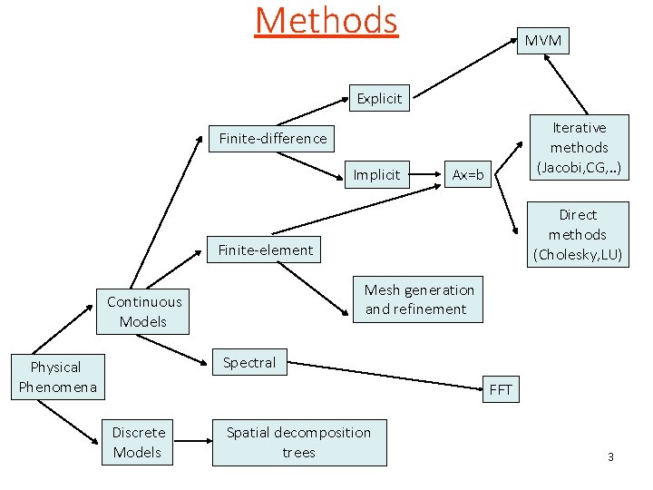
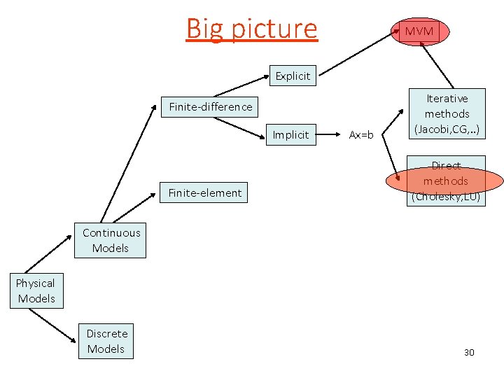
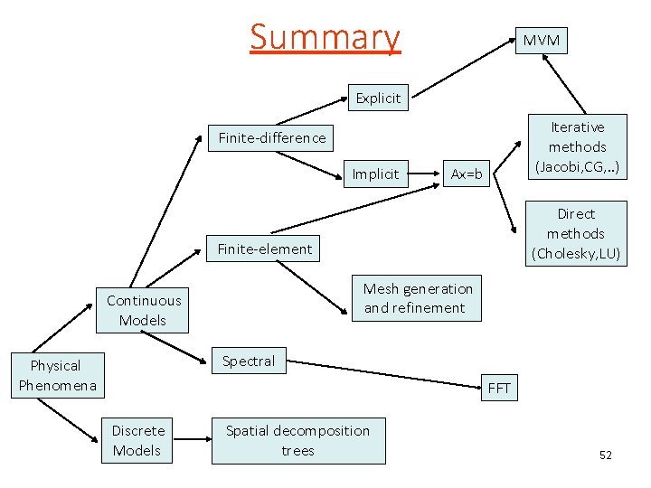
Methods MVM Explicit Iterative methods (Jacobi, CG, . . ) Finite-difference Implicit Ax=b Direct methods (Cholesky, LU) Finite-element Mesh generation and refinement Continuous Models Spectral Physical Phenomena FFT Discrete Models Spatial decomposition trees 3

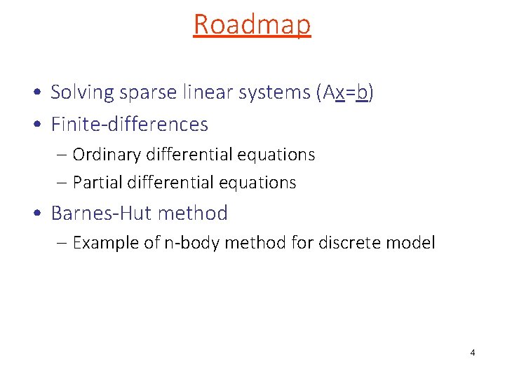
Roadmap • Solving sparse linear systems (Ax=b) • Finite-differences – Ordinary differential equations – Partial differential equations • Barnes-Hut method – Example of n-body method for discrete model 4

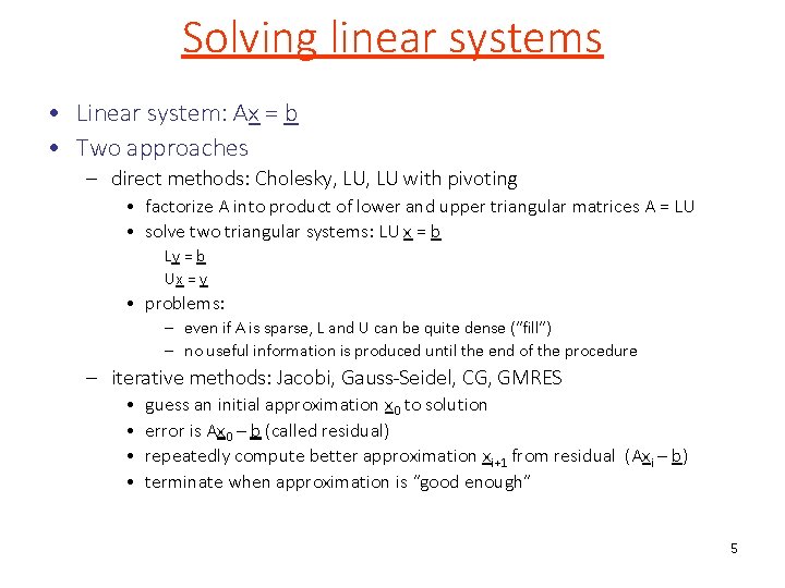
Solving linear systems • Linear system: Ax = b • Two approaches – direct methods: Cholesky, LU with pivoting • factorize A into product of lower and upper triangular matrices A = LU • solve two triangular systems: LU x = b Ly = b Ux = y • problems: – even if A is sparse, L and U can be quite dense (“fill”) – no useful information is produced until the end of the procedure – iterative methods: Jacobi, Gauss-Seidel, CG, GMRES • • guess an initial approximation x 0 to solution error is Ax 0 – b (called residual) repeatedly compute better approximation xi+1 from residual (Axi – b) terminate when approximation is “good enough” 5

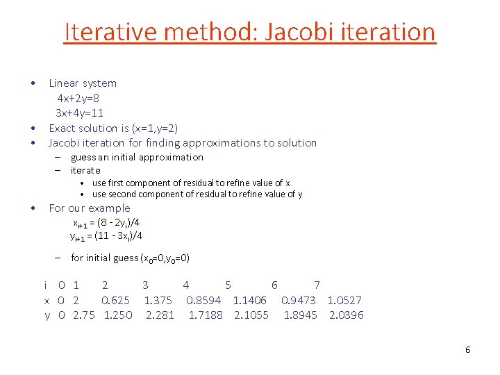
Iterative method: Jacobi iteration • Linear system 4 x+2 y=8 3 x+4 y=11 • Exact solution is (x=1, y=2) • Jacobi iteration for finding approximations to solution – guess an initial approximation – iterate • use first component of residual to refine value of x • use second component of residual to refine value of y • For our example xi+1 = (8 - 2 yi)/4 yi+1 = (11 - 3 xi)/4 – for initial guess (x 0=0, y 0=0) i 0 1 2 3 4 5 6 7 x 0 2 0. 625 1. 375 0. 8594 1. 1406 0. 9473 1. 0527 y 0 2. 75 1. 250 2. 281 1. 7188 2. 1055 1. 8945 2. 0396 6

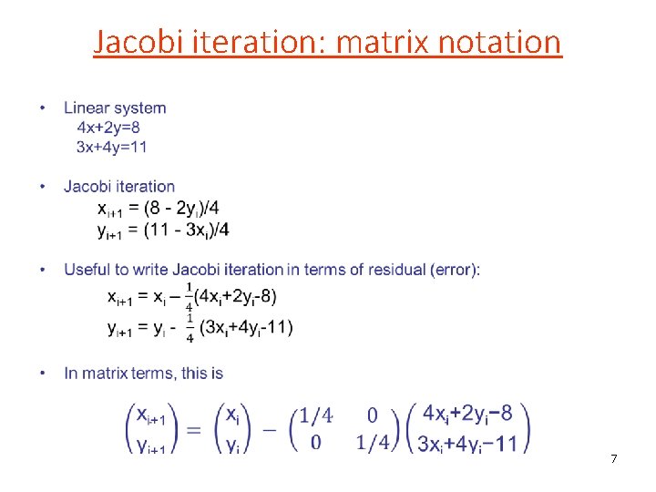
Jacobi iteration: matrix notation • 7

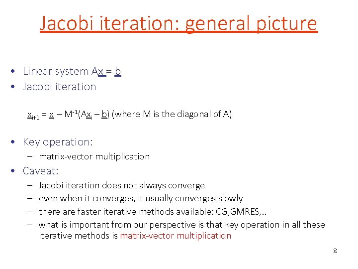
Jacobi iteration: general picture • Linear system Ax = b • Jacobi iteration xi+1 = xi – M-1(Axi – b) (where M is the diagonal of A) • Key operation: – matrix-vector multiplication • Caveat: – – Jacobi iteration does not always converge even when it converges, it usually converges slowly there are faster iterative methods available: CG, GMRES, . . what is important from our perspective is that key operation in all these iterative methods is matrix-vector multiplication 8

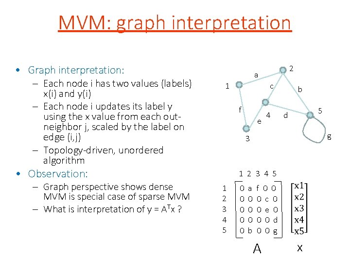
MVM: graph interpretation • Graph interpretation: – Each node i has two values (labels) x(i) and y(i) – Each node i updates its label y using the x value from each outneighbor j, scaled by the label on edge (i, j) – Topology-driven, unordered algorithm 1 c f e 4 b 5 d g 3 • Observation: – Graph perspective shows dense MVM is special case of sparse MVM – What is interpretation of y = ATx ? 2 a 1 2 3 4 5 0 0 0 a 0 0 0 b f 0 0 0 c 0 0 e 0 0 0 d 0 0 g A x

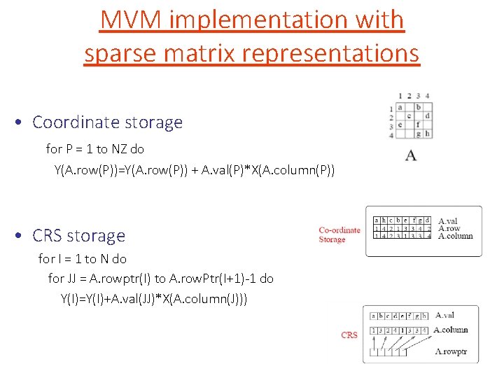
MVM implementation with sparse matrix representations • Coordinate storage for P = 1 to NZ do Y(A. row(P))=Y(A. row(P)) + A. val(P)*X(A. column(P)) • CRS storage for I = 1 to N do for JJ = A. rowptr(I) to A. row. Ptr(I+1)-1 do Y(I)=Y(I)+A. val(JJ)*X(A. column(J)))

Finite-differences 11

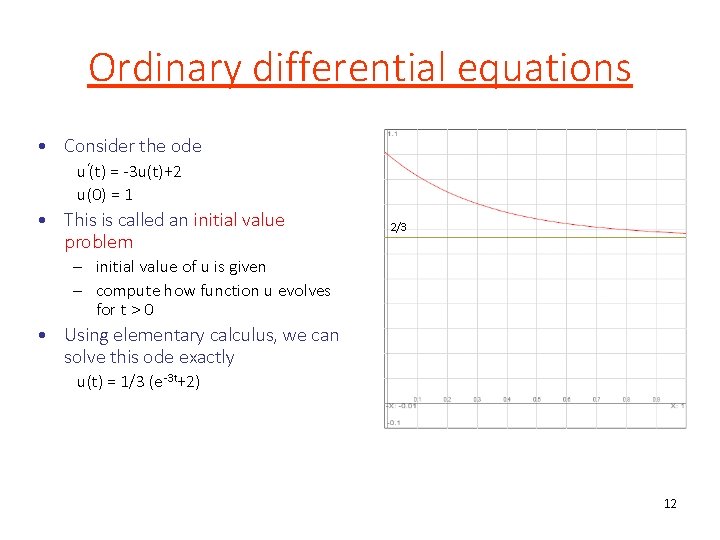
Ordinary differential equations • Consider the ode u‘(t) = -3 u(t)+2 u(0) = 1 • This is called an initial value problem 2/3 – initial value of u is given – compute how function u evolves for t > 0 • Using elementary calculus, we can solve this ode exactly u(t) = 1/3 (e-3 t+2) 12

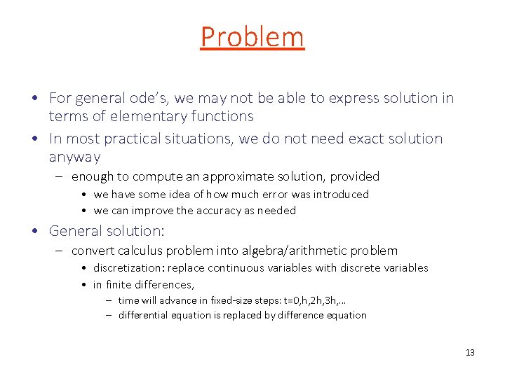
Problem • For general ode’s, we may not be able to express solution in terms of elementary functions • In most practical situations, we do not need exact solution anyway – enough to compute an approximate solution, provided • we have some idea of how much error was introduced • we can improve the accuracy as needed • General solution: – convert calculus problem into algebra/arithmetic problem • discretization: replace continuous variables with discrete variables • in finite differences, – time will advance in fixed-size steps: t=0, h, 2 h, 3 h, … – differential equation is replaced by difference equation 13

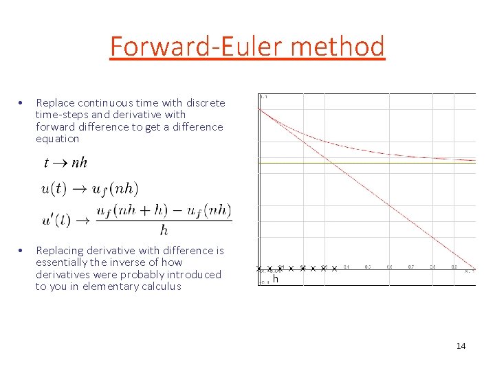
Forward-Euler method • Replace continuous time with discrete time-steps and derivative with forward difference to get a difference equation • Replacing derivative with difference is essentially the inverse of how derivatives were probably introduced to you in elementary calculus x x x x h 14

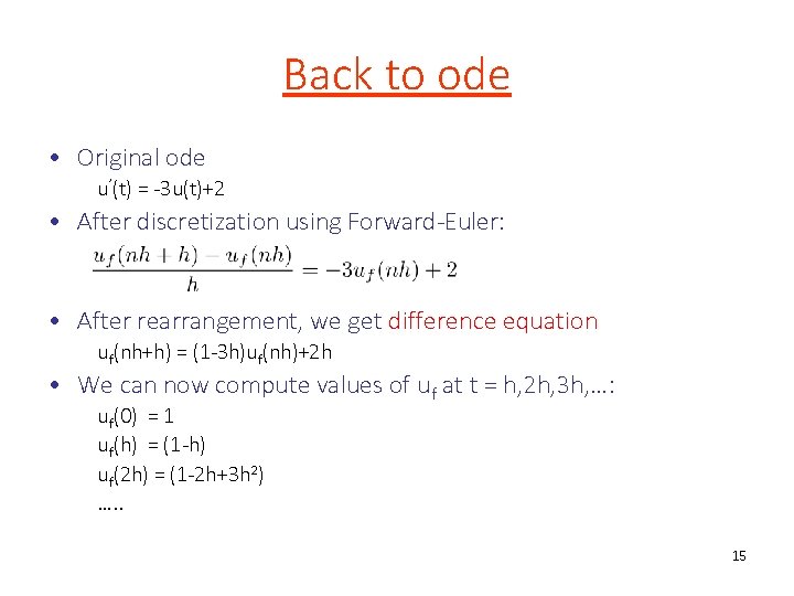
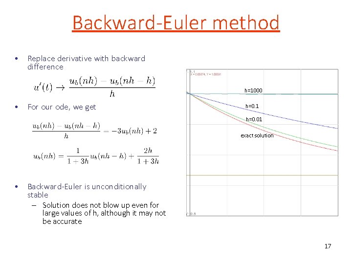
Back to ode • Original ode u’(t) = -3 u(t)+2 • After discretization using Forward-Euler: • After rearrangement, we get difference equation uf(nh+h) = (1 -3 h)uf(nh)+2 h • We can now compute values of uf at t = h, 2 h, 3 h, …: uf(0) = 1 uf(h) = (1 -h) uf(2 h) = (1 -2 h+3 h 2) …. . 15

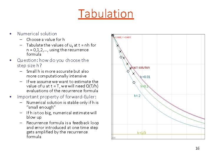
Tabulation • Numerical solution – Choose a value for h – Tabulate the values of uf at t = nh for n = 0, 1, 2, …, using the recurrence formula • Question: how do you choose the step size h? – Small h is more accurate but also more computationally intensive – If we assume we want to estimate the value of u at t = T, we will need O(T/h) evaluations of the recurrence formula • Important property of forward-Euler: – Numerical solution is stable only if h is “small enough” – If h is too big, numerical estimate will blow up – Recurrence formula is a feedback loop and error introduced at one time step gets amplified by the recurrence formula ox x xexact solution o x h=0. 01 o h=0. 1 h=. 2 h=1/3 16

Backward-Euler method • Replace derivative with backward difference h=1000 • For our ode, we get h=0. 1 h=0. 01 exact solution • Backward-Euler is unconditionally stable – Solution does not blow up even for large values of h, although it may not be accurate 17

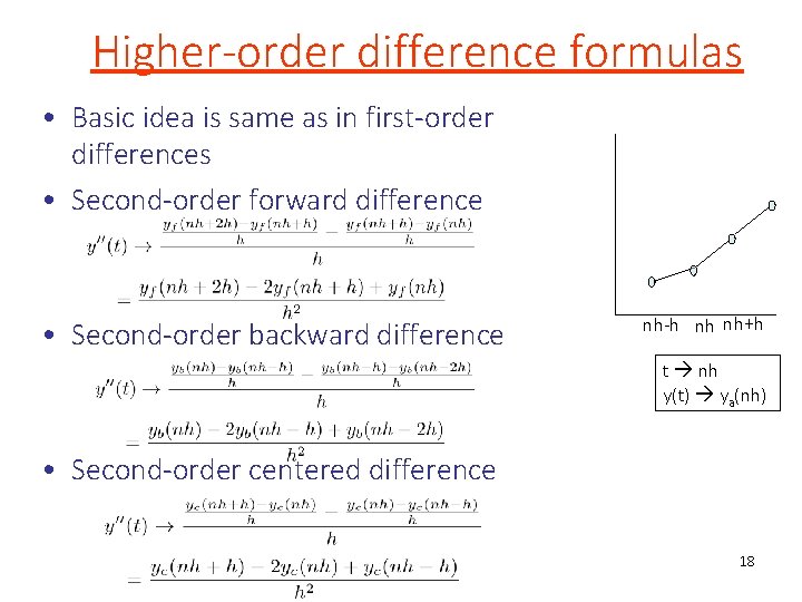
Higher-order difference formulas • Basic idea is same as in first-order differences • Second-order forward difference • Second-order backward difference nh-h nh nh+h t nh y(t) ya(nh) • Second-order centered difference 18

General comments • Many other discretization schemes have been developed in literature (e. g. Runge-Kutta) • Figures of merit for discretization schemes – Stability: can approximate solution blow up? – Accuracy: how small does step size have to be for approximate solution to be “close enough” to exact solution? • Obvious extension to systems of ode’s – Backward-Euler and centered differences require solution of linear systems at each time-step. – Forward-Euler does not. – Sometimes known as implicit and explicit methods; implicit methods require linear solves at each time-step. 19

Finite-differences: partial differential equations 20

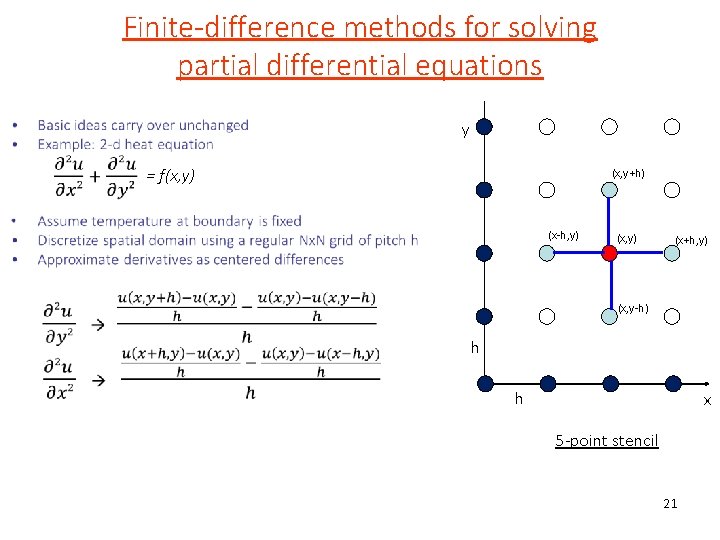
Finite-difference methods for solving partial differential equations y = f(x, y) (x, y+h) (x-h, y) (x+h, y) (x, y-h) h h x 5 -point stencil 21

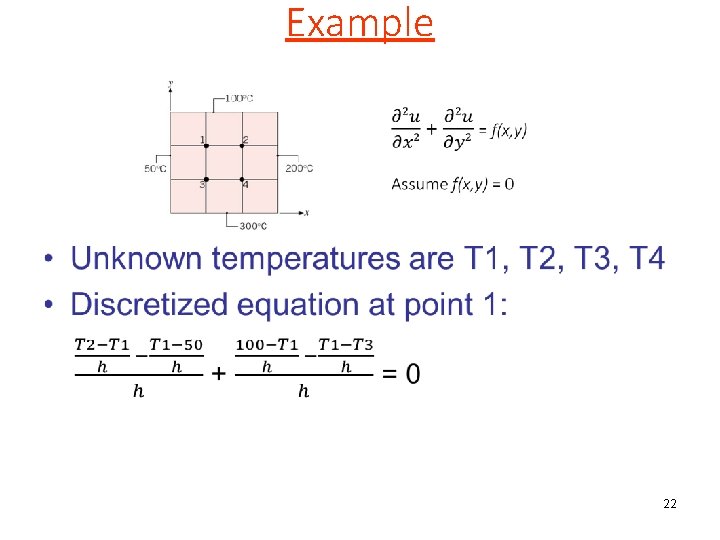
Example • 22

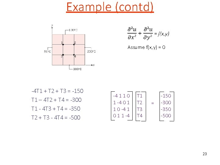
Example (contd) Assume f(x, y) = 0 -4 T 1 + T 2 + T 3 = -150 T 1 – 4 T 2 + T 4 = -300 T 1 - 4 T 3 + T 4 = -350 T 2 + T 3 - 4 T 4 = -500 -4 1 1 0 1 -4 0 1 1 0 -4 1 0 1 1 -4 T 1 T 2 T 3 T 4 = -150 -300 -350 -500 23

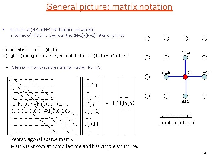
General picture: matrix notation • System of (N-1)x(N-1) difference equations in terms of the unknowns at the (N-1)x(N-1) interior points for all interior points (ih, jh) u(ih, jh+h)+u(ih, jh-h)+u(ih+h, jh)+u(ih-h, jh) – 4 u(ih, jh) = h 2 f(ih, jh) • Matrix notation: use natural order for u’s ……………………………… 0. . 1 0. . 0 1 -4 1 0. . 0 1 0… 0. 0. . 0 0 1 0. . 0 1 -4 1 0. . 0 1 0. ………………………………. . . …. u(i-1, j) …. u(i, j-1) u(i, j+1). . . u(i+1, j) …… (i, j+1) (i-1, j) ……. = h 2 f(ih, jh) ……. . (i, j) (i+1, j) (i, j-1) 5 -point stencil (matrix indices) Pentadiagonal sparse matrix Matrix is known at compile-time and has simple structure. 24

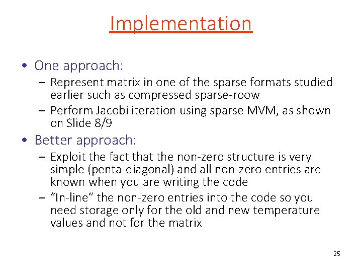
Implementation • One approach: – Represent matrix in one of the sparse formats studied earlier such as compressed sparse-roow – Perform Jacobi iteration using sparse MVM, as shown on Slide 8/9 • Better approach: – Exploit the fact that the non-zero structure is very simple (penta-diagonal) and all non-zero entries are known when you are writing the code – “In-line” the non-zero entries into the code so you need storage only for the old and new temperature values and not for the matrix 25

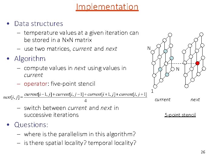
Implementation • Data structures – temperature values at a given iteration can be stored in a Nx. N matrix – use two matrices, current and next N • Algorithm – compute values in next using values in current – operator: five-point stencil N 1 current – switch between current and next in successive iterations next 5 -point stencil • Questions: – where is the parallelism in this algorithm? – is there spatial locality? temporal locality? 26

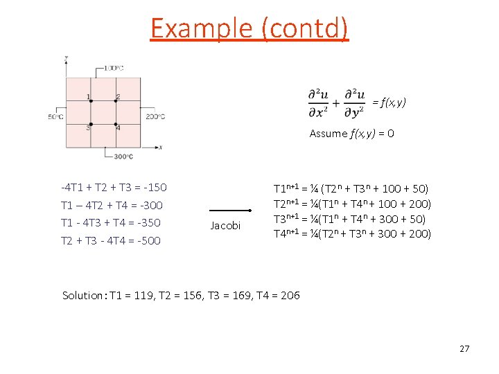
Example (contd) = f(x, y) Assume f(x, y) = 0 -4 T 1 + T 2 + T 3 = -150 T 1 – 4 T 2 + T 4 = -300 T 1 - 4 T 3 + T 4 = -350 T 2 + T 3 - 4 T 4 = -500 Jacobi T 1 n+1 = ¼ (T 2 n + T 3 n + 100 + 50) T 2 n+1 = ¼(T 1 n + T 4 n + 100 + 200) T 3 n+1 = ¼(T 1 n + T 4 n + 300 + 50) T 4 n+1 = ¼(T 2 n + T 3 n + 300 + 200) Solution: T 1 = 119, T 2 = 156, T 3 = 169, T 4 = 206 27

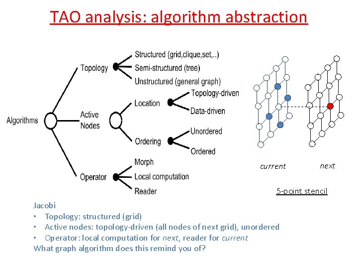
TAO analysis: algorithm abstraction current next 5 -point stencil Jacobi • Topology: structured (grid) • Active nodes: topology-driven (all nodes of next grid), unordered • Operator: local computation for next, reader for current What graph algorithm does this remind you of?

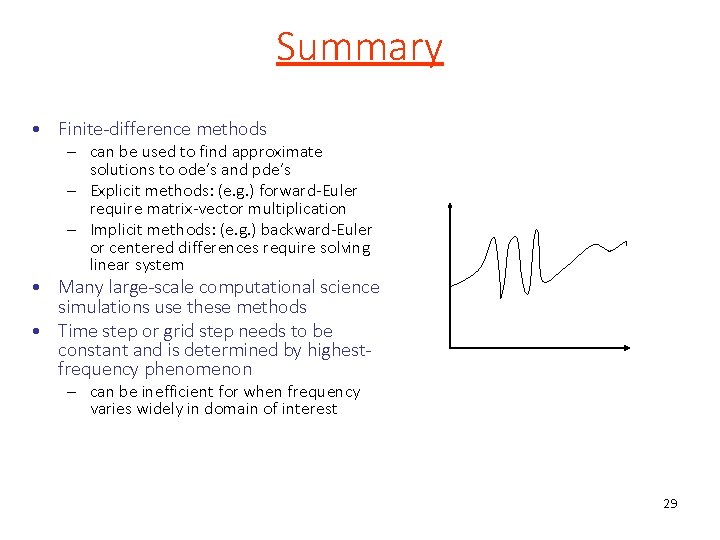
Summary • Finite-difference methods – can be used to find approximate solutions to ode’s and pde’s – Explicit methods: (e. g. ) forward-Euler require matrix-vector multiplication – Implicit methods: (e. g. ) backward-Euler or centered differences require solving linear system • Many large-scale computational science simulations use these methods • Time step or grid step needs to be constant and is determined by highestfrequency phenomenon – can be inefficient for when frequency varies widely in domain of interest 29

Big picture MVM Explicit Finite-difference Implicit Finite-element Ax=b Iterative methods (Jacobi, CG, . . ) Direct methods (Cholesky, LU) Continuous Models Physical Models Discrete Models 30

Discrete models: Barnes Hut algorithm

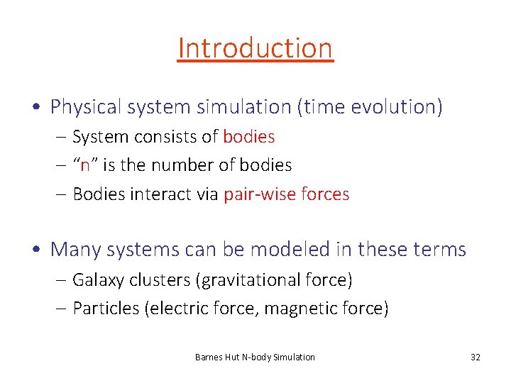
Introduction • Physical system simulation (time evolution) – System consists of bodies – “n” is the number of bodies – Bodies interact via pair-wise forces • Many systems can be modeled in these terms – Galaxy clusters (gravitational force) – Particles (electric force, magnetic force) Barnes Hut N-body Simulation 32

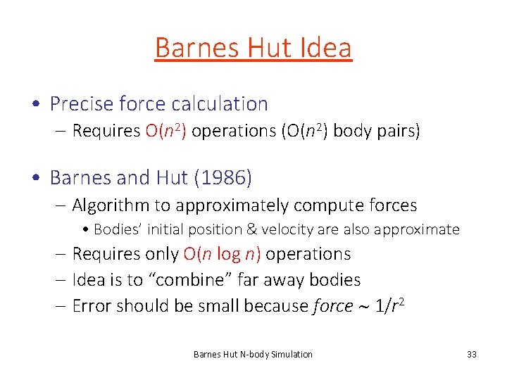
Barnes Hut Idea • Precise force calculation – Requires O(n 2) operations (O(n 2) body pairs) • Barnes and Hut (1986) – Algorithm to approximately compute forces • Bodies’ initial position & velocity are also approximate – Requires only O(n log n) operations – Idea is to “combine” far away bodies – Error should be small because force 1/r 2 Barnes Hut N-body Simulation 33

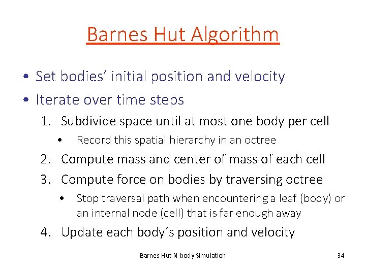
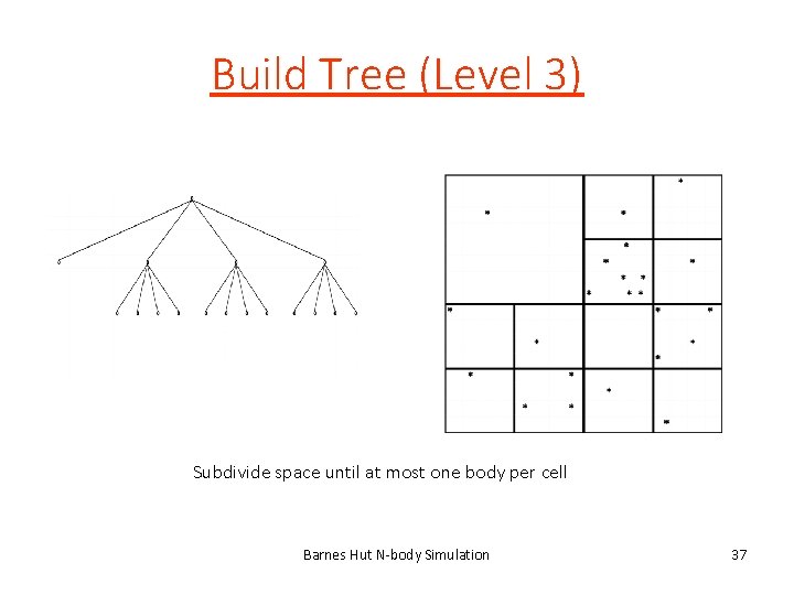
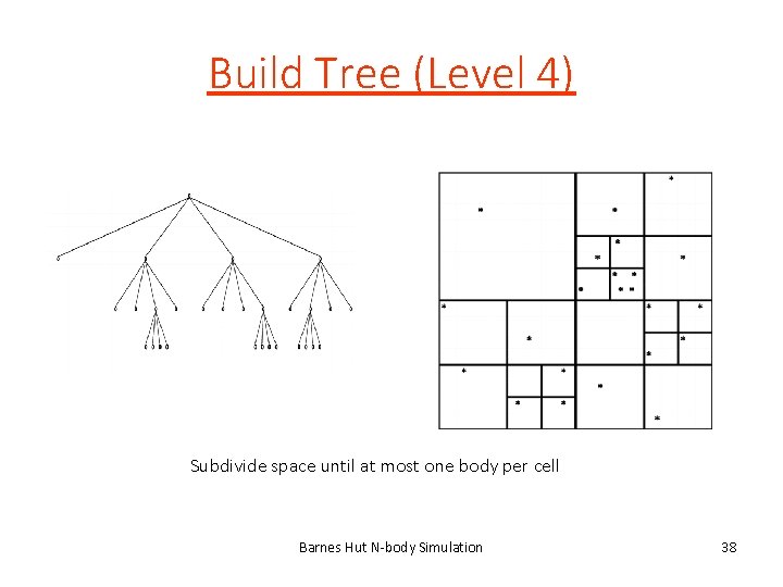
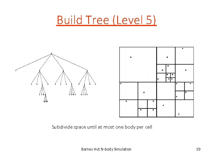
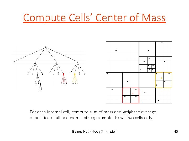
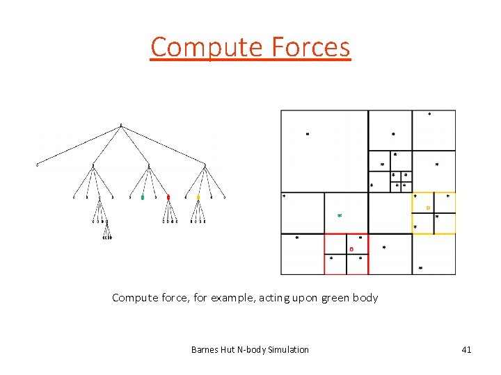
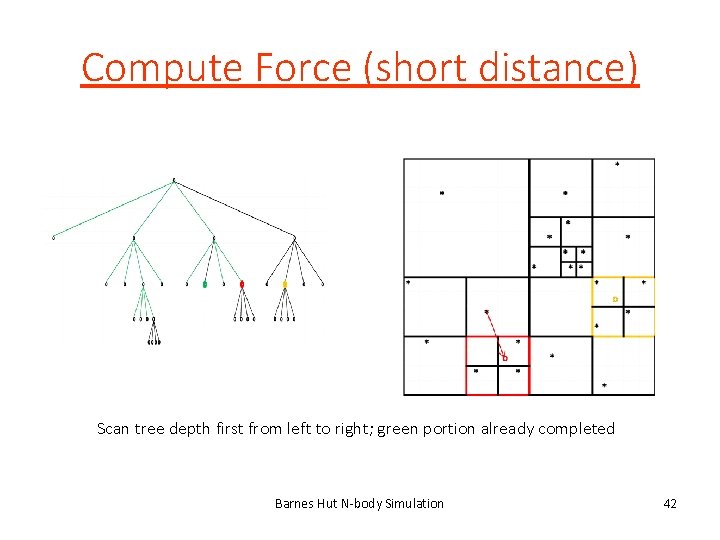
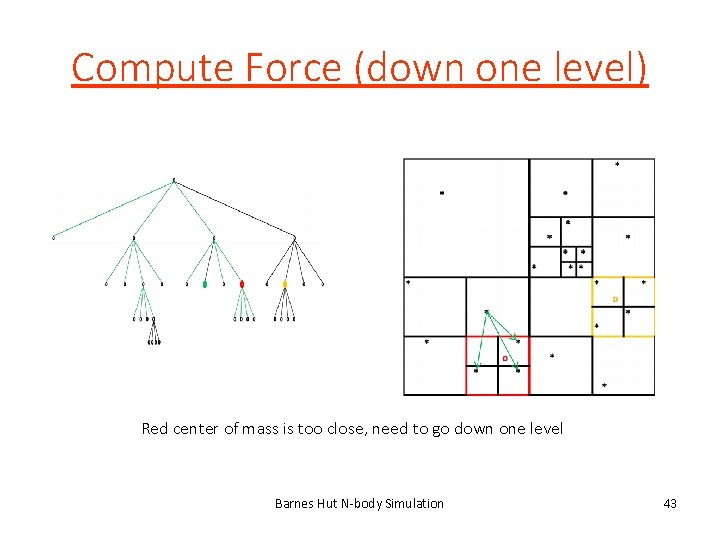
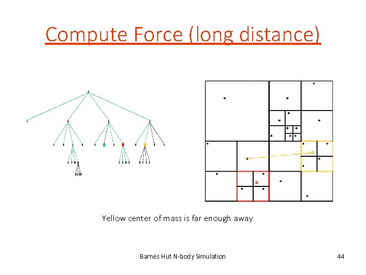
Barnes Hut Algorithm • Set bodies’ initial position and velocity • Iterate over time steps 1. Subdivide space until at most one body per cell • Record this spatial hierarchy in an octree 2. Compute mass and center of mass of each cell 3. Compute force on bodies by traversing octree • Stop traversal path when encountering a leaf (body) or an internal node (cell) that is far enough away 4. Update each body’s position and velocity Barnes Hut N-body Simulation 34

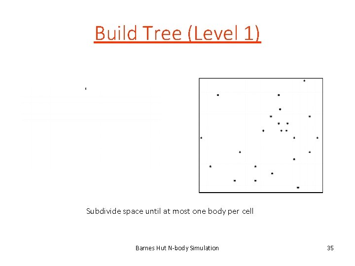
Build Tree (Level 1) Subdivide space until at most one body per cell Barnes Hut N-body Simulation 35

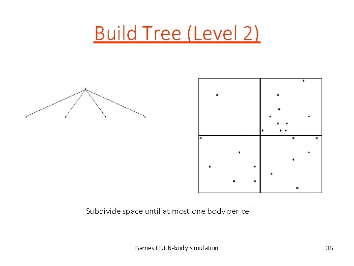
Build Tree (Level 2) Subdivide space until at most one body per cell Barnes Hut N-body Simulation 36

Build Tree (Level 3) Subdivide space until at most one body per cell Barnes Hut N-body Simulation 37

Build Tree (Level 4) Subdivide space until at most one body per cell Barnes Hut N-body Simulation 38

Build Tree (Level 5) Subdivide space until at most one body per cell Barnes Hut N-body Simulation 39

Compute Cells’ Center of Mass For each internal cell, compute sum of mass and weighted average of position of all bodies in subtree; example shows two cells only Barnes Hut N-body Simulation 40

Compute Forces Compute force, for example, acting upon green body Barnes Hut N-body Simulation 41

Compute Force (short distance) Scan tree depth first from left to right; green portion already completed Barnes Hut N-body Simulation 42

Compute Force (down one level) Red center of mass is too close, need to go down one level Barnes Hut N-body Simulation 43

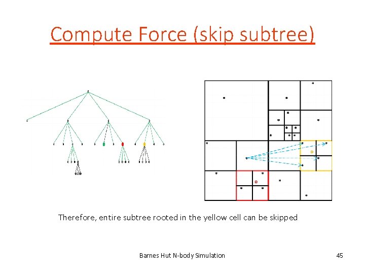
Compute Force (long distance) Yellow center of mass is far enough away Barnes Hut N-body Simulation 44

Compute Force (skip subtree) Therefore, entire subtree rooted in the yellow cell can be skipped Barnes Hut N-body Simulation 45

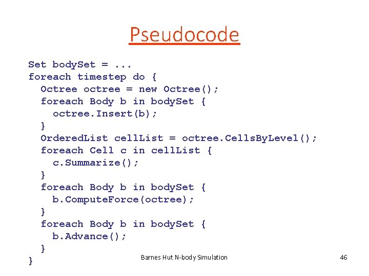
Pseudocode Set body. Set =. . . foreach timestep do { Octree octree = new Octree(); foreach Body b in body. Set { octree. Insert(b); } Ordered. List cell. List = octree. Cells. By. Level(); foreach Cell c in cell. List { c. Summarize(); } foreach Body b in body. Set { b. Compute. Force(octree); } foreach Body b in body. Set { b. Advance(); } Barnes Hut N-body Simulation } 46

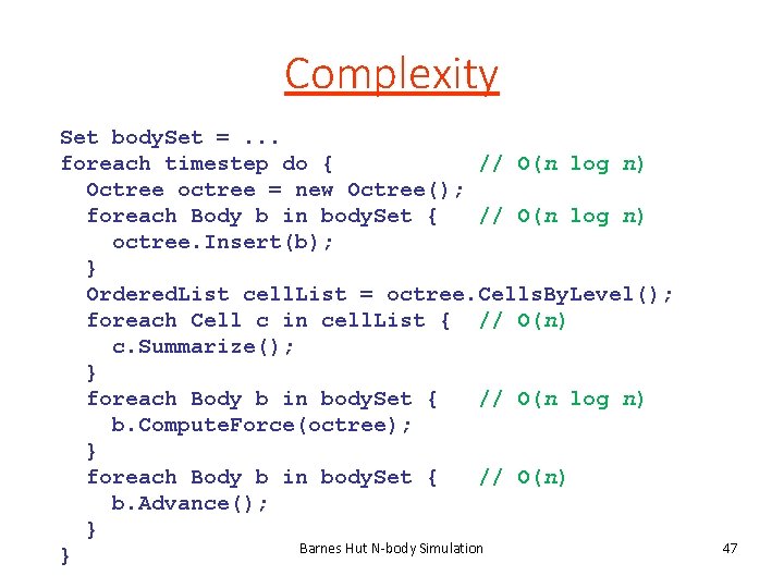
Complexity Set body. Set =. . . foreach timestep do { // O(n log n) Octree octree = new Octree(); foreach Body b in body. Set { // O(n log n) octree. Insert(b); } Ordered. List cell. List = octree. Cells. By. Level(); foreach Cell c in cell. List { // O(n) c. Summarize(); } foreach Body b in body. Set { // O(n log n) b. Compute. Force(octree); } foreach Body b in body. Set { // O(n) b. Advance(); } Barnes Hut N-body Simulation } 47

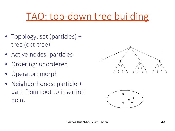
TAO: top-down tree building • Topology: set (particles) + tree (oct-tree) • Active nodes: particles • Ordering: unordered • Operator: morph • Neighborhoods: particle + path from root to insertion point Barnes Hut N-body Simulation 48

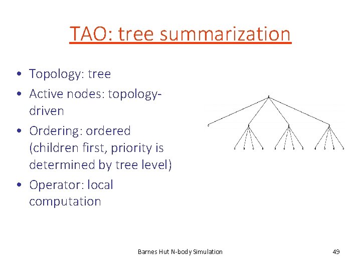
TAO: tree summarization • Topology: tree • Active nodes: topologydriven • Ordering: ordered (children first, priority is determined by tree level) • Operator: local computation Barnes Hut N-body Simulation 49

TAO: force computation • • Topology: tree (oct-tree) + set (particles) Active nodes: particles Ordering: unordered Operator: reader + local computation Barnes Hut N-body Simulation 50

TAO: Advancing bodies • • Topology: set (particles) Active nodes: particles Operator: local computation Ordering: unordered Barnes Hut N-body Simulation 51

Summary MVM Explicit Iterative methods (Jacobi, CG, . . ) Finite-difference Implicit Ax=b Direct methods (Cholesky, LU) Finite-element Mesh generation and refinement Continuous Models Spectral Physical Phenomena FFT Discrete Models Spatial decomposition trees 52