Computational Physics ZCE 111 Yoon Tiem Leong USM

Computational Physics (ZCE 111) Yoon Tiem Leong USM School of Physics, Academic Year 2010/11, 2 nd semester

Note The lecture notes are adopted from Giodarno and Nakanishi, Second edition. Programming tool: Mathematica Install your own Mathematica. For instruction, visit the course webpage. Visit the course webpage and to read more about what’s computational physics. Read Giodano.

Chapter 1 A First Numerical Problem

1. 1 Radioactive Decay A large sample of nuclei decays according to the first order equation The analytical solution is given by where t is the mean lifetime for a particular nuclear species. Plot the graph using Mathematica's Plot command. [Sample code 1. 1. 1] In order to plot the graph, numerical values must be supplied to N U (0) and t. These are the ‘initial values’. For example, U-238, t = 10 9 yr. Note that to plot the function, you must not use the symbol "N" to name the function, since "N" is the symbol reserved for Mathematica. Use the symbol "Nu" instead of "N" (it's just a label anyway).

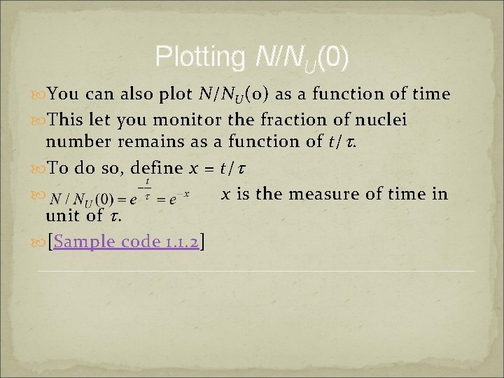
Plotting N/NU(0) You can also plot N/N U (0) as a function of time This let you monitor the fraction of nuclei number remains as a function of t/ t. To do so, define x = t/ t x is the measure of time in unit of t. [Sample code 1. 1. 2]

Estimating the half life Can you estimate the time (in unit of t ) when the half of the original nuclei has decayed? Theoretically, this time is called the half-life, given by e -t/ t = 1/2, i. e. , t t 1/2 = t ln 2, or x = t/t = ln 2. How to obtain t 1/2 using Mathematica? This could be solved using the function Solve. Here we ask the Mathematica to solve the equation for the value of t such that f(t)= e -t/ t = ½. [Sample code 1. 1. 3]

Try this What is the time t' taken for 75% of the total nuclei has decayed? This means only 35% = 0. 35 of the nuclei remains at time t'. To solve for t' in Mathematica, see Sample code 1. 1. 4.

Improved the way to use Solve A slightly more improved way to use the Solve function can be found in Sample code 1. 1. 5 tprime= t /. Solve[Exp[-t/tau] == frac, t] [[1]] Here tprime is the numerical value of the solution to the equation Exp[-t/tau] == frac, where frac = 0. 35 in our case.

DSolve Mathematica's DSolve function can be used to solve the differential equation d. N/dt=-(N/ t ). This is a symbolic operation. Sample code 1. 1. 6.

NDSolve Mathematica's NDSolve function can be used to solve the equation d. N/dt=-(N/ t ). This is a numerical operation. Sample code 1. 1. 7. To use NDSolve, numerical values of the initial or boundary conditions for the differential equation must be supplied, e. g. , Nu[0]==N 0.

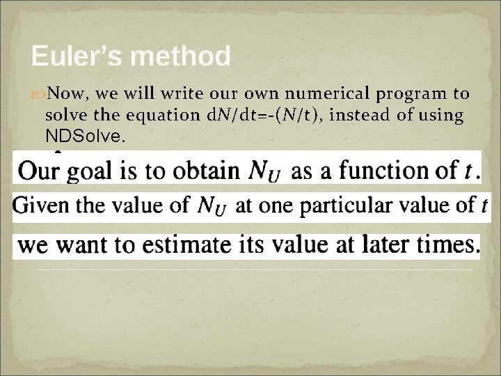
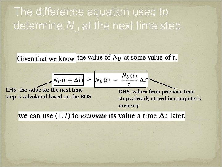
Euler’s method Now, we will write our own numerical program to solve the equation d. N/dt=-(N/t), instead of using NDSolve.

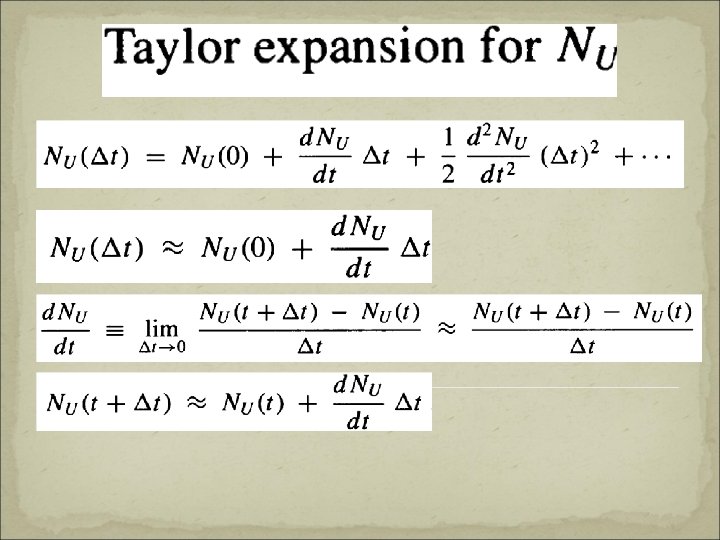
The difference equation used to determine NU at the next time step LHS, the value for the next time step is calculated based on the RHS, values from previous time steps already stored in computer’s memory

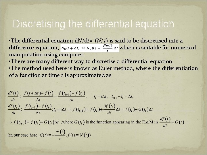
Discretising the differential equation • The differential equation d. N/dt=-(N/t) is said to be discretised into a difference equation, which is suitable for numerical manipulation using computer. • There are many different way to discretise a differential equation. • The method used here is known as Euler method, where the differentiation of a function at time t is approximated as

General structure of a code Initialisation Calculation Output

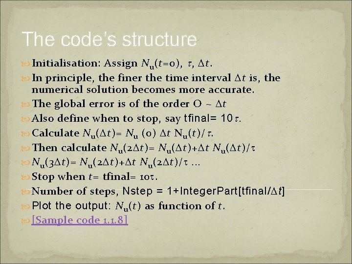
The code’s structure Initialisation: Assign N u (t=0), t , Dt. In principle, the finer the time interval Dt is, the numerical solution becomes more accurate. The global error is of the order O ~ Dt Also define when to stop, say tfinal= 10 t. Calculate N u (Dt)= N u (0) Dt N u (t)/ t. Then calculate N u (2 Dt)= N u (Dt)+Dt N u (Dt)/t N u (3 Dt)= N u (2 Dt)+Dt N u (2 Dt)/t. . . Stop when t= tfinal= 10 t. Number of steps, Nstep = 1+Integer. Part[tfinal/Dt] Plot the output: N u (t) as function of t. [Sample code 1. 1. 8]