Computational Physics Lecture 19 PHY 4061 Using neural

Computational Physics (Lecture 19) PHY 4061

Using neural nets to recognize handwritten digits • http: //neuralnetworksanddeeplearning. com/c hap 1. html

• Consider the following sequence of handwritten digits • Effortless to recognize those digits as 504192. • Deceptive ease. – humans have a primary visual cortex, • Also known as V 1, containing 140 million neurons, • Tens of billions of connections between them!

• Darwin: Development of the eye as a significant difficulty for his theory of evolution by natural selection. • In The Origin of Species: – To suppose that the eye, with all its inimitable contrivances. . could have been formed by natural selection, seems, I freely confess, absurd in the highest possible degree.

• human vision involves not just V 1, – an entire series of visual cortices • V 2, V 3, V 4, and V 5 – doing progressively more complex image processing. • A supercomputer in our heads – Tuned by evolution over hundreds of millions of years – Superbly adapted to understand the visual world. – Recognizing handwritten digits isn't easy. • But nearly all that work is done unconsciously. • And so we don't usually appreciate how tough a problem our visual systems solve.

Rule based strategy • "a 9 has a loop at the top, and a vertical stroke in the bottom right" – – Not so simple to express algorithmically. – To make such rules precise, • you quickly get lost in a morass of exceptions and caveats and special cases. • hopeless.

Neural networks approach • Take a large number of handwritten digits, known as training examples

• Develop a system – learn from those training examples. • Uses the examples to automatically infer rules • the network can learn more about handwriting, and so improve its accuracy by increasing the training samples. • We could build a better handwriting recognizer by using thousands or even millions or billions of training examples.

Goal of this chapter • Implementing a neural network – to recognize handwritten digits. • The program is just 74 lines long without special neural network libraries. • But this short program can recognize digits with an accuracy over 96 percent, without human intervention.

Perceptrons • Developed in the 1950 s and 1960 s – by Frank Rosenblatt, inspired by earlier work by Warren Mc. Culloch and Walter Pitts. • Today, it's more common to use other models of artificial neurons • In much modern work on neural networks, the main neuron model used the sigmoid neuron.

How do perceptrons work? • A perceptron takes several binary inputs, x 1, x 2…. , and produces a single binary output:

• Rosenblatt proposed a simple rule to compute the output. • Weights, w 1, w 2, … – real numbers expressing the importance of the respective inputs to the output. – The neuron's output, 0 or 1, is determined by whether the weighted sum ∑jwjxj is less than or greater than some threshold value. – Just like the weights, the threshold is a real number which is a parameter of the neuron. • output= 0 if ∑jwjxj≤ threshold 1 if ∑jwjxj > threshold

One example • There's going to be a cheese festival in your city. – Whether or not to go? • Make your decision by weighing up three factors: – Is the weather good? – Does your boyfriend or girlfriend want to accompany you? – Is the festival near public transit? (You don't own a car).

• We can represent these three factors by x 1, x 2 and x 3. • For instance, we'd have x 1=1 if the weather is good, x 1=0 if the weather is bad. – x 2=1 if your boyfriend or girlfriend wants to go, and x 2=0 if not. And similarly again for x 3 and public transit.

• Suppose you absolutely adore cheese – You're happy to go to the festival even if your boyfriend or girlfriend is uninterested and the festival is hard to get to. – Perhaps you really loathe bad weather, and there's no way you'd go to the festival if the weather is bad. – You can use perceptrons to model this kind of decision-making.

• One way to do this is to choose a weight w 1=6 for the weather, and w 2=2 and w 3=2 for the other conditions. • Now you see an example of importance sampling. • The larger value of w 1 => • the weather matters a lot to you Suppose you choose a threshold of 5 for the perceptron. • With these choices, the perceptron implements the desired decision-making model, • Outputting 1 whenever the weather is good, and 0 whenever the weather is bad.

• Varying the weights and the threshold, – we can get different models of decision-making. • Suppose we instead chose a threshold of 3. – The perceptron would decide that you should go to the festival whenever the weather was good or when both the festival was near public transit and your boyfriend or girlfriend was willing to join you. • It'd be a different model of decision-making. • Dropping the threshold means you're more willing to go to the festival.

• The example illustrates is how a perceptron can weigh up different kinds of evidence in order to make decisions. • And it should seem plausible that a complex network of perceptrons could make quite subtle decisions:

• In this network, the first column of perceptrons – The first layer of perceptrons • is making three very simple decisions. – Each of those perceptrons in the second layer is making a decision by weighing up the results from the first layer of decision-making. – In this way a perceptron in the second layer can make a decision at a more complex and more abstract level than perceptrons in the first layer. – And even more complex decisions can be made by the perceptron in the third layer. In this way, a many-layer network of perceptrons can engage in sophisticated decision making.

• Two notational changes. • To write ∑jwjxj as a dot product, w⋅x≡∑jwjxj, where w and x are vectors – whose components are the weights and inputs, respectively. • To move threshold to the other side of the inequality, – replace it by what's known as the perceptron's bias, • b≡−threshold. • the perceptron rule can be rewritten: – output= 0, if w⋅x+b≤ 0 1, if w⋅x+b>0

• Bias – a measure of how easy it is to get the perceptron to output a 1. – Or a measure of how easy it is to get the perceptron to fire. – A really big bias, • extremely easy to output a 1. – Very negative, • difficult to output a 1.

• Another Usage of perceptrons – to compute the elementary logical functions • For example, suppose we have a perceptron with two inputs, each with weight − 2, and an overall bias of 3. Here's our perceptron:

• • Input 0 0 produces output 1, Inputs 0 1 and 1 0 produce output 1 Input 1 1 produces output 0, And so our perceptron implements a NAND gate! – Therefore all the logical gates in your computer form a subset of perceptrons.

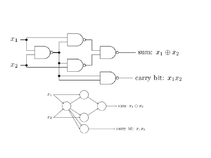
• The NAND example shows – we can use perceptrons to compute simple logical functions. – In fact, we can use networks of perceptrons to compute any logical function at all. – For example, we can use NAND gates to build a circuit which adds two bits, x 1 and x 2. This requires computing the bitwise sum, x 1⊕x 2, as well as a carry bit which is set to 1 when both x 1 and x 2 are 1, i. e. , the carry bit is just the bitwise product x 1 x 2:

• One notable aspect of this network – The output from the leftmost perceptron is used twice as input to the bottommost perceptron. • If we don't want to allow this kind of thing, – it's possible to simply merge the two lines, into a single connection with a weight of -4 instead of two connections with -2 weights.

• it's conventional to draw an extra layer of perceptrons - the input layer- to encode the inputs:

• The adder example demonstrates how a network of perceptrons can be used to simulate a circuit containing many NAND gates. – Because NAND gates are universal for computation, it follows that perceptrons are also universal for computation. • The computational universality of perceptrons is simultaneously reassuring and disappointing. – Reassuring • It tells us that networks of perceptrons can be as powerful as any other computing device. – Disappointing, • it seem as though perceptrons are merely a new type of NAND gate.

• We can devise learning algorithms – which can automatically tune the weights and biases of a network of artificial neurons. • This tuning happens in response to external stimuli, without direct intervention by a programmer. • These learning algorithms enable us to use artificial neurons in a way which is radically different to conventional logic gates. • Our neural networks can simply learn to solve problems!

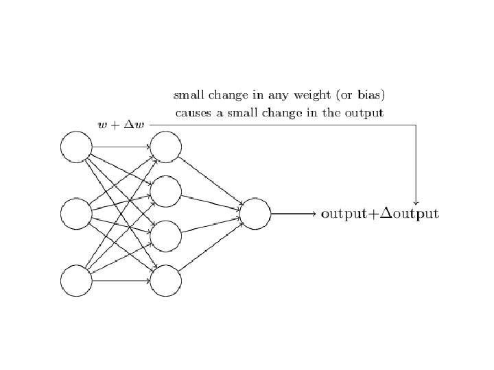
Sigmoid neurons • Suppose we have a network of perceptrons that we'd like to use to learn to solve some problem. • The inputs to the network might be the raw pixel data from a scanned, handwritten image of a digit. • And we'd like the network to learn weights and biases so that the output from the network correctly classifies the digit. • To see how learning might work, suppose we make a small change in some weight (or bias) in the network. What we'd like is for this small change in weight to cause only a small corresponding change in the output from the network. • This property will make learning possible. – What if small change in weight lead to a big change in the output, or small change in weight lead to no change in the output?

• If it were true that a small change in a weight (or bias) causes only a small change in output, – then we could use this fact to modify the weights and biases to get our network to behave more in the manner we want. • For example, suppose the network was mistakenly classifying an image as an "8" when it should be a "9". • We could figure out how to make a small change in the weights and biases so the network gets a little closer to classifying the image as a "9". And then we'd repeat this, changing the weights and biases over and over to produce better and better output. The network would be learning. – An iterative procedure!

• The problem – this isn't what happens when our network contains perceptrons. • A small change in the weights or bias of any single perceptron in the network can sometimes cause the output of that perceptron to completely flip! – From 0 to 1. • That flip may then cause the behavior of the rest of the network to completely change in some very complicated way. • While your "9" might now be classified correctly, the behavior of the network on all the other images is likely to have completely changed in some hard-to-control way. • That makes it difficult to see how to gradually modify the weights and biases so that the network gets closer to the desired behavior.

• We can overcome this problem by introducing a new type of artificial neuron called a sigmoid neuron. • Sigmoid neurons are similar to perceptrons, but modified so that small changes in their weights and bias cause only a small change in their output. • That's the crucial fact which will allow a network of sigmoid neurons to learn.

• Just like a perceptron, the sigmoid neuron has inputs, x 1, x 2, … • Instead of being just 0 or 1, these inputs can also take on any values between 0 and 1. – So, for instance, 0. 638… is a valid input for a sigmoid neuron. • Also just like a perceptron, the sigmoid neuron has weights for each input, w 1, w 2, • And an overall bias, b. But the output is not 0 or 1. • Instead, it's σ(w⋅x+b), where σ is called the sigmoid function • Incidentally, σ is sometimes called the logistic function, and this new class of neurons called logistic neurons. • σ(z)≡ 1/ (1+e−z).

• To put it all a little more explicitly, – the output of a sigmoid neuron • with inputs x 1, x 2, …, • weights w 1, w 2, …, • and bias b is 1/(1+exp(−∑jwjxj−b)). • At first sight, sigmoid neurons appear very different to perceptrons. – The algebraic form of the sigmoid function may seem opaque and forbidding if you're not already familiar with it. – In fact, there are many similarities between perceptrons and sigmoid neurons, and the algebraic form of the sigmoid function turns out to be more of a technical detail than a true barrier to understanding.

• Suppose z≡w⋅x+b is a large positive number. – Then e−z≈0 – and so σ(z)≈1. – In other words, when z=w⋅x+b is large and positive, • the output from the sigmoid neuron is approximately 1 • just as it would have been for a perceptron. • Suppose on the other hand that z=w⋅x+b is very negative. – Then e−z→∞, – and σ(z)≈0. So when z=w⋅x+b is very negative, the behavior of a sigmoid neuron also closely approximates a perceptron. • It's only when w⋅x+b is of modest size that there's much deviation from the perceptron model.

• In fact, the exact form of σ isn't so important - what really matters is the shape of the function when plotted. Here's the shape:

• smoothed out version of a step function:

• If σ had in fact been a step function, then the sigmoid neuron would be a perceptron, since the output would be 1 or 0 depending on whether w⋅x+b was positive or negative • So, strictly speaking, we'd need to modify the step function at that one point. But you get the idea. . By using the actual σ function we get, as already implied above, a smoothed out perceptron. • Indeed, it's the smoothness of the σ function that is the crucial fact, not its detailed form. • The smoothness of σ means that small changes Δwj in the weights and Δb in the bias will produce a small change Δoutput in the output from the neuron.

• Δoutput is well approximated by – Δoutput≈∑j(∂output/∂wj)Δwj+(∂output/∂b)Δb • Δoutput is a linear function of the changes Δwj and Δb in the weights and bias. • This linearity makes it easy to choose small changes in the weights and biases to achieve any desired small change in the output. • So while sigmoid neurons have much of the same qualitative behaviour as perceptrons, they make it much easier to figure out how changing the weights and biases will change the output.

• One big difference between perceptrons and sigmoid neurons – sigmoid neurons don't just output 0 or 1. • They can have as output any real number between 0 and 1 • Useful If we want to use the output value to represent the average intensity of the pixels in an image input to a neural network. • But sometimes it can be a nuisance. – Suppose we want the output from the network to indicate either "the input image is a 9” or "the input image is not a 9". – Obviously, it'd be easiest to do this if the output was a 0 or a 1, as in a perceptron. – But in practice we can set up a convention to deal with this, for example, by deciding to interpret any output of at least 0. 5 as indicating a "9", and any output less than 0. 5 as indicating "not a 9".

The architecture of neural networks

• The design of the input and output layers in a network is often straightforward. • For example, suppose we're trying to determine whether a handwritten image depicts a "9" or not. • A natural way to design the network is to encode the intensities of the image pixels into the input neurons. • If the image is a 64 by 64 greyscale image, – then we'd have 4, 096 input neurons, with the intensities scaled appropriately between 0 and 1. – The output layer will contain just a single neuron, with output values of less than 0. 5 indicating "input image is not a 9", – and values greater than 0. 5 indicating "input image is a 9 ".

• While the design of the input and output layers of a neural network is often straightforward, there can be quite an art to the design of the hidden layers. • In particular, it's not possible to sum up the design process for the hidden layers with a few simple rules of thumb. • Instead, neural networks researchers have developed many design heuristics for the hidden layers, which help people get the behavior they want out of their nets. • For example, such heuristics can be used to help determine how to trade off the number of hidden layers against the time required to train the network.

• Neural networks where the output from one layer is used as input to the next layer. – feedforward neural networks. • This means there are no loops in the network – information is always fed forward, never fed back. – If we did have loops, we'd end up with situations where the input to the σ function depended on the output. That'd be hard to make sense of, and so we don't allow such loops. – Current and future strongly couple with each other!

• However, there are other models of artificial neural networks in which feedback loops are possible. These models are called recurrent neural networks. – The idea in these models is to have neurons which fire for some limited duration of time, before becoming quiescent. – That firing can stimulate other neurons, which may fire a little while later, also for a limited duration. – That causes still more neurons to fire, and so over time we get a cascade of neurons firing. – Loops don't cause problems in such a model, since a neuron's output only affects input at some later time, not instantaneously.

• Recurrent neural nets have been less influential than feedforward networks, in part because the learning algorithms for recurrent nets are (at least to date) less powerful. • But recurrent networks are still extremely interesting. – They're much closer in spirit to how our brains work than feedforward networks. – And it's possible that recurrent networks can solve important problems which can only be solved with great difficulty by feedforward networks.

A simple network to classify handwritten digits • Split the problem into two sub-problems. – First, breaking an image containing many digits into a sequence of separate images, • each containing a single digit. • For example, break the image • into

• humans solve this segmentation problem with ease • challenging for a computer program to correctly break up the image. • Next, the program needs to classify each individual digit. – So, for instance, to recognize that the first digit above, , is 5.

• We'll focus on classifying individual digits. – because segmentation problem is not so difficult • Many approaches to solving the segmentation problem. – One approach: to trial many different ways of segmenting the image – Using the individual digit classifier to score each trial segmentation.

• A trial segmentation gets a high score – if the individual digit classifier is confident of its classification in all segments, – a low score if the classifier is having a lot of trouble in one or more segments. – The idea is that if the classifier is having trouble somewhere, then it's probably having trouble because the segmentation has been chosen incorrectly. – This idea and other variations can be used to solve the segmentation problem quite well. • So instead of worrying about segmentation we'll concentrate on developing a neural network which can solve the more interesting and difficult problem, namely, recognizing individual handwritten digits.