Computational meshes matrices conjugate gradients and mesh partitioning

Computational meshes, matrices, conjugate gradients, and mesh partitioning Some slides are from David Culler, Jim Demmel, Bob Lucas, Horst Simon, Kathy Yelick, et al. , UCB CS 267

Parallelism in Regular meshes • Computing a Stencil on a regular mesh • need to communicate mesh points near boundary to neighboring processors. • Often done with ghost regions • Surface-to-volume ratio keeps communication down, but • Still may be problematic in practice Implemented using “ghost” regions. Adds memory overhead 2

Irregular mesh: NASA Airfoil in 2 D 3

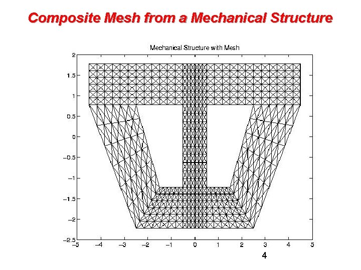
Composite Mesh from a Mechanical Structure 4

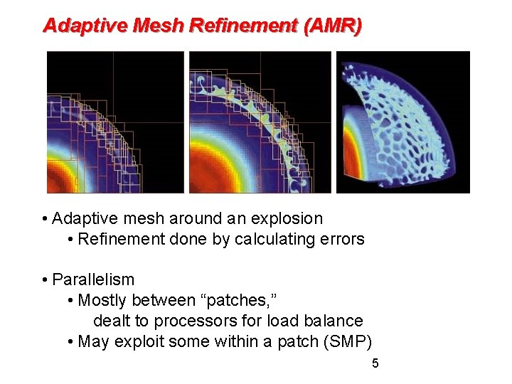
Adaptive Mesh Refinement (AMR) • Adaptive mesh around an explosion • Refinement done by calculating errors • Parallelism • Mostly between “patches, ” dealt to processors for load balance • May exploit some within a patch (SMP) 5

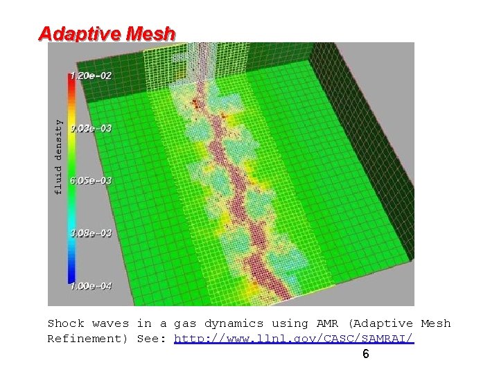
fluid density Adaptive Mesh Shock waves in a gas dynamics using AMR (Adaptive Mesh Refinement) See: http: //www. llnl. gov/CASC/SAMRAI/ 6

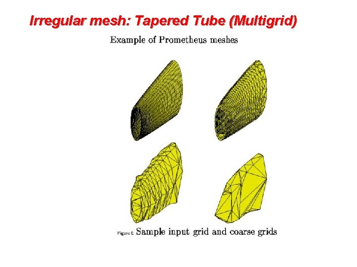
Irregular mesh: Tapered Tube (Multigrid) 7

Challenges of Irregular Meshes for PDE’s • How to generate them in the first place • E. g. Triangle, a 2 D mesh generator by Jonathan Shewchuk • 3 D harder! E. g. QMD by Stephen Vavasis • How to partition them • Par. Metis, a parallel graph partitioner • How to design iterative solvers • PETSc, a Portable Extensible Toolkit for Scientific Computing • Prometheus, a multigrid solver for finite element problems on irregular meshes • How to design direct solvers • Super. LU, parallel sparse Gaussian elimination • These are challenges to do sequentially, more so in parallel 8

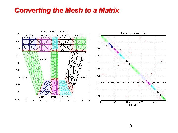
Converting the Mesh to a Matrix 9

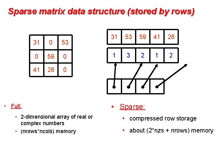
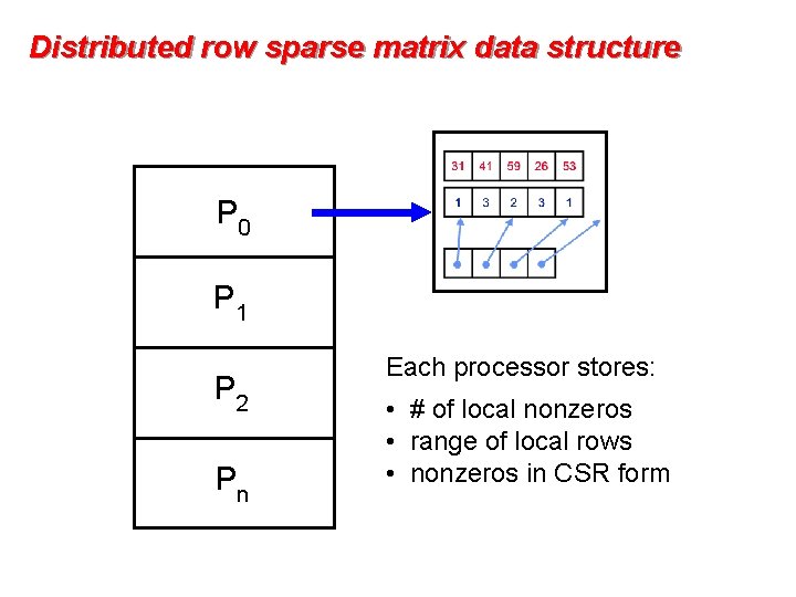
Sparse matrix data structure (stored by rows) 31 0 53 0 59 0 41 26 0 • Full: • 2 -dimensional array of real or complex numbers • (nrows*ncols) memory 31 53 59 41 26 1 3 2 1 2 • Sparse: • compressed row storage • about (2*nzs + nrows) memory

Distributed row sparse matrix data structure P 0 P 1 P 2 Pn Each processor stores: • # of local nonzeros • range of local rows • nonzeros in CSR form

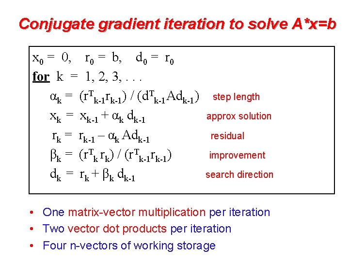
Conjugate gradient iteration to solve A*x=b x 0 = 0, r 0 = b, d 0 = r 0 for k = 1, 2, 3, . . . αk = (r. Tk-1 rk-1) / (d. Tk-1 Adk-1) xk = xk-1 + αk dk-1 rk = rk-1 – αk Adk-1 βk = (r. Tk rk) / (r. Tk-1 rk-1) dk = rk + βk dk-1 step length approx solution residual improvement search direction • One matrix-vector multiplication per iteration • Two vector dot products per iteration • Four n-vectors of working storage

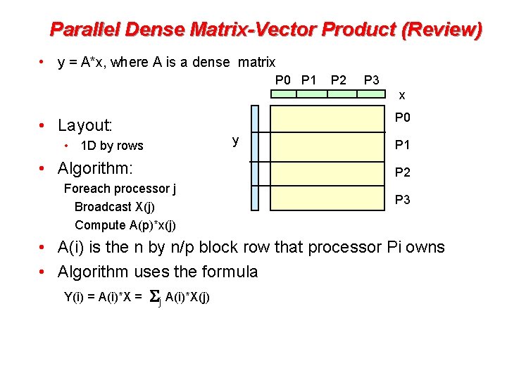
Parallel Dense Matrix-Vector Product (Review) • y = A*x, where A is a dense matrix P 0 P 1 P 2 P 3 x • Layout: • 1 D by rows • Algorithm: Foreach processor j Broadcast X(j) Compute A(p)*x(j) P 0 y P 1 P 2 P 3 • A(i) is the n by n/p block row that processor Pi owns • Algorithm uses the formula Y(i) = A(i)*X = Sj A(i)*X(j)

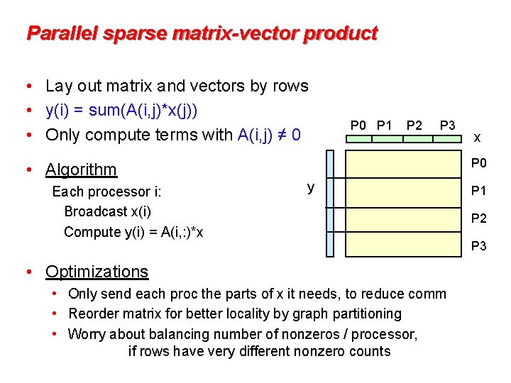
Parallel sparse matrix-vector product • Lay out matrix and vectors by rows • y(i) = sum(A(i, j)*x(j)) • Only compute terms with A(i, j) ≠ 0 • Algorithm Each processor i: Broadcast x(i) Compute y(i) = A(i, : )*x P 0 P 1 P 2 P 3 x P 0 y • Optimizations • Only send each proc the parts of x it needs, to reduce comm • Reorder matrix for better locality by graph partitioning • Worry about balancing number of nonzeros / processor, if rows have very different nonzero counts P 1 P 2 P 3

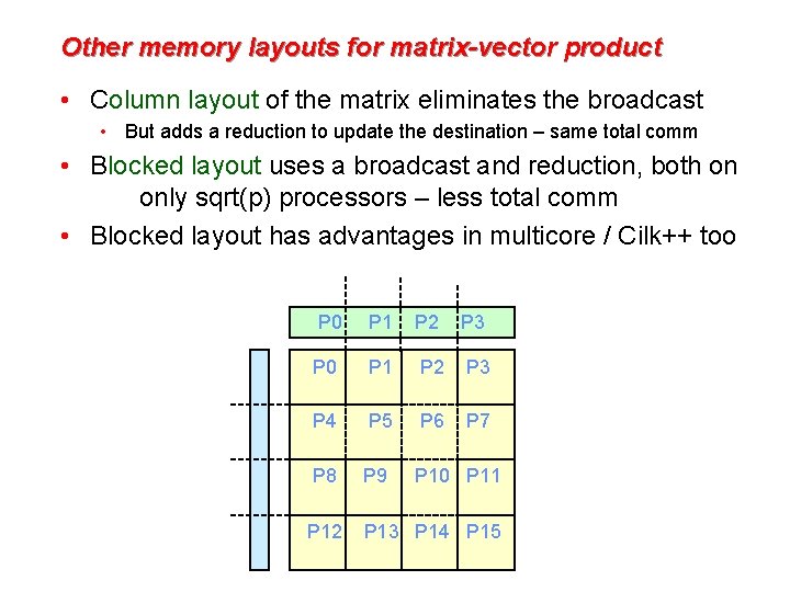
Other memory layouts for matrix-vector product • Column layout of the matrix eliminates the broadcast • But adds a reduction to update the destination – same total comm • Blocked layout uses a broadcast and reduction, both on only sqrt(p) processors – less total comm • Blocked layout has advantages in multicore / Cilk++ too P 0 P 1 P 2 P 3 P 4 P 5 P 6 P 7 P 8 P 9 P 10 P 11 P 12 P 13 P 14 P 15

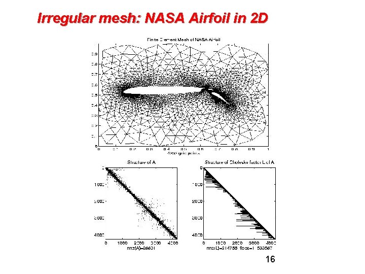
Irregular mesh: NASA Airfoil in 2 D 16

Graphs and Sparse Matrices • Sparse matrix is a representation of a (sparse) graph 1 1 2 6 5 6 1 1 3 5 4 1 2 1 4 3 1 1 4 1 1 1 2 3 1 1 6 5 • Matrix entries are edge weights • Number of nonzeros per row is the vertex degree • Edges represent data dependencies in matrix-vector multiplication

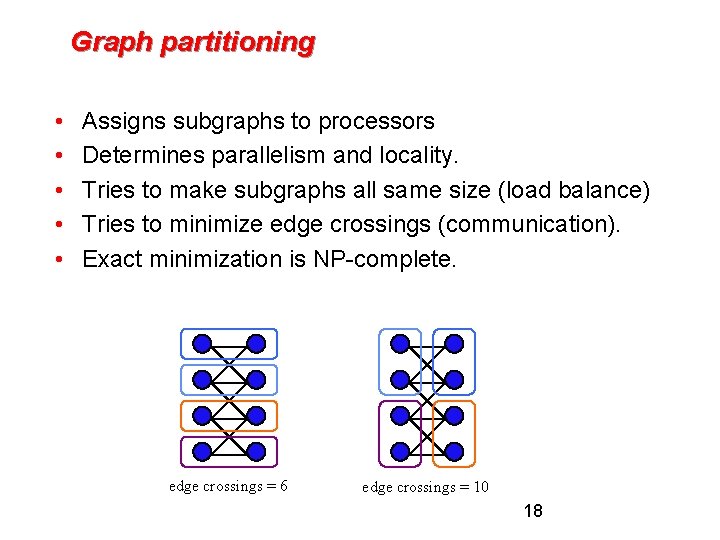
Graph partitioning • • • Assigns subgraphs to processors Determines parallelism and locality. Tries to make subgraphs all same size (load balance) Tries to minimize edge crossings (communication). Exact minimization is NP-complete. edge crossings = 6 edge crossings = 10 18

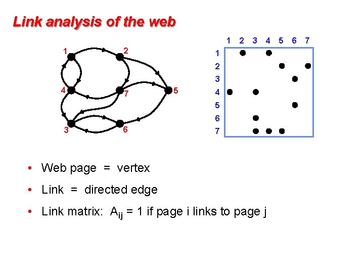
Link analysis of the web 1 1 2 2 3 4 1 2 3 4 7 5 4 5 6 3 6 7 • Web page = vertex • Link = directed edge • Link matrix: Aij = 1 if page i links to page j 5 6 7

Web graph: Page. Rank (Google) [Brin, Page] An important page is one that many important pages point to. • Markov process: follow a random link most of the time; otherwise, go to any page at random. • Importance = stationary distribution of Markov process. • Transition matrix is p*A + (1 -p)*ones(size(A)), scaled so each column sums to 1. • Importance of page i is the i-th entry in the principal eigenvector of the transition matrix. • But the matrix is 1, 000, 000 by 1, 000, 000.

A Page Rank Matrix • Importance ranking of web pages • Stationary distribution of a Markov chain • Power method: matvec and vector arithmetic • Matlab*P page ranking demo (from SC’ 03) on a web crawl of mit. edu (170, 000 pages)

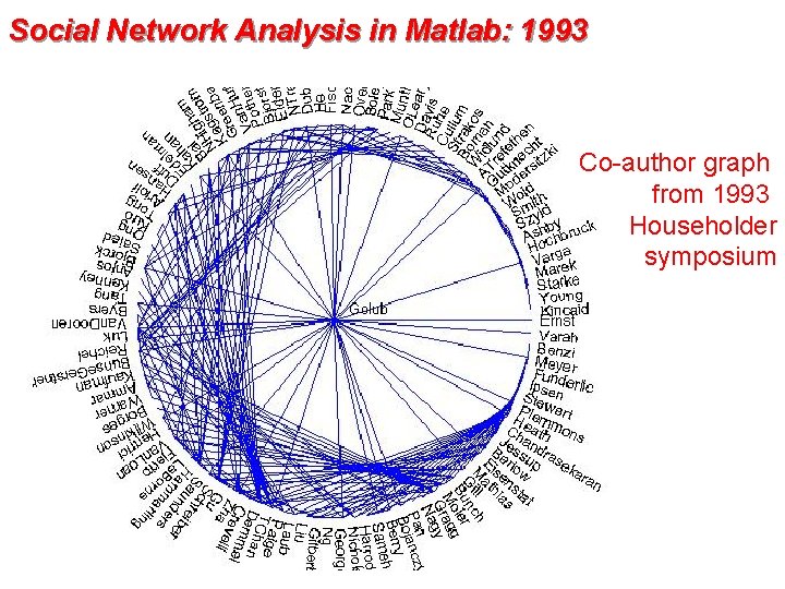
Social Network Analysis in Matlab: 1993 Co-author graph from 1993 Householder symposium

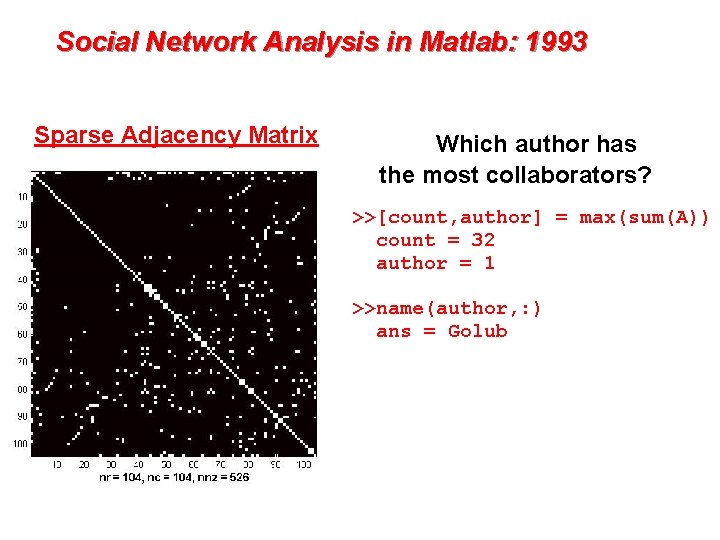
Social Network Analysis in Matlab: 1993 Sparse Adjacency Matrix Which author has the most collaborators? >>[count, author] = max(sum(A)) count = 32 author = 1 >>name(author, : ) ans = Golub

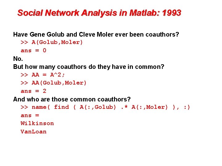
Social Network Analysis in Matlab: 1993 Have Gene Golub and Cleve Moler ever been coauthors? >> A(Golub, Moler) ans = 0 No. But how many coauthors do they have in common? >> AA = A^2; >> AA(Golub, Moler) ans = 2 And who are those common coauthors? >> name( find ( A(: , Golub). * A(: , Moler) ), : ) ans = Wilkinson Van. Loan