Computational Intelligence Winter Term 201718 Prof Dr Gnter

Computational Intelligence Winter Term 2017/18 Prof. Dr. Günter Rudolph Lehrstuhl für Algorithm Engineering (LS 11) Fakultät für Informatik TU Dortmund

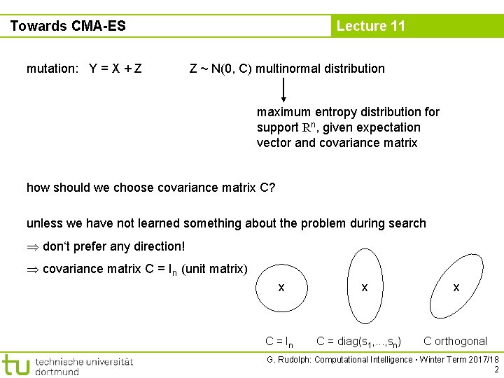
Towards CMA-ES mutation: Y = X + Z Lecture 11 Z ~ N(0, C) multinormal distribution maximum entropy distribution for support Rn, given expectation vector and covariance matrix how should we choose covariance matrix C? unless we have not learned something about the problem during search don‘t prefer any direction! covariance matrix C = In (unit matrix) x C = In x C = diag(s 1, . . . , sn) x C orthogonal G. Rudolph: Computational Intelligence ▪ Winter Term 2017/18 2

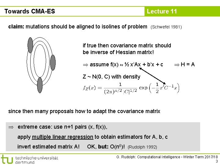
Towards CMA-ES Lecture 11 claim: mutations should be aligned to isolines of problem (Schwefel 1981) if true then covariance matrix should be inverse of Hessian matrix! assume f(x) ½ x‘Ax + b‘x + c H=A Z ~ N(0, C) with density since then many proposals how to adapt the covariance matrix extreme case: use n+1 pairs (x, f(x)), apply multiple linear regression to obtain estimators for A, b, c invert estimated matrix A! OK, but: O(n 6)! (Rudolph 1992) G. Rudolph: Computational Intelligence ▪ Winter Term 2017/18 3

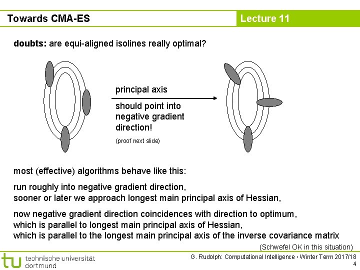
Towards CMA-ES Lecture 11 doubts: are equi-aligned isolines really optimal? principal axis should point into negative gradient direction! (proof next slide) most (effective) algorithms behave like this: run roughly into negative gradient direction, sooner or later we approach longest main principal axis of Hessian, now negative gradient direction coincidences with direction to optimum, which is parallel to longest main principal axis of Hessian, which is parallel to the longest main principal axis of the inverse covariance matrix (Schwefel OK in this situation) G. Rudolph: Computational Intelligence ▪ Winter Term 2017/18 4

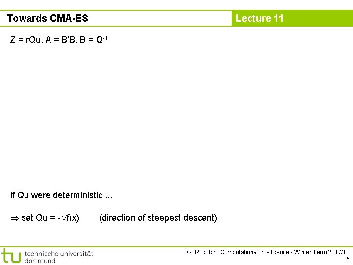
Towards CMA-ES Lecture 11 Z = r. Qu, A = B‘B, B = Q-1 if Qu were deterministic. . . set Qu = - f(x) (direction of steepest descent) G. Rudolph: Computational Intelligence ▪ Winter Term 2017/18 5

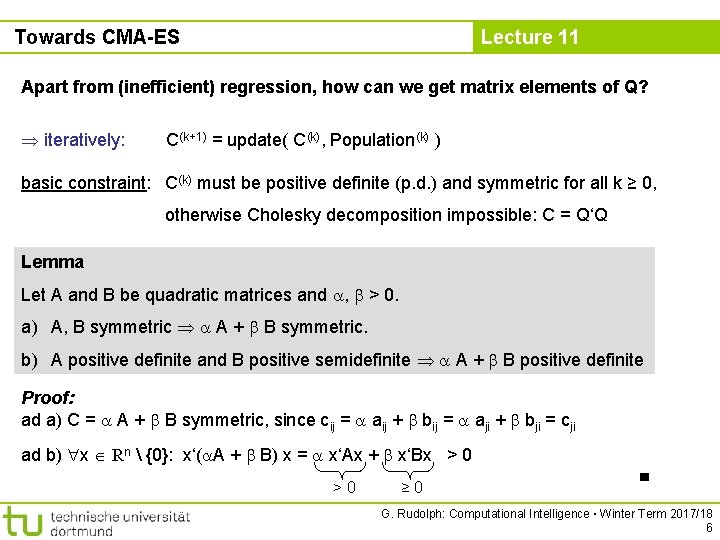
Towards CMA-ES Lecture 11 Apart from (inefficient) regression, how can we get matrix elements of Q? iteratively: C(k+1) = update( C(k), Population(k) ) basic constraint: C(k) must be positive definite (p. d. ) and symmetric for all k ≥ 0, otherwise Cholesky decomposition impossible: C = Q‘Q Lemma Let A and B be quadratic matrices and , > 0. a) A, B symmetric A + B symmetric. b) A positive definite and B positive semidefinite A + B positive definite Proof: ad a) C = A + B symmetric, since cij = aij + bij = aji + bji = cji ad b) x Rn {0}: x‘( A + B) x = x‘Ax + x‘Bx > 0 >0 ≥ 0 ■ G. Rudolph: Computational Intelligence ▪ Winter Term 2017/18 6

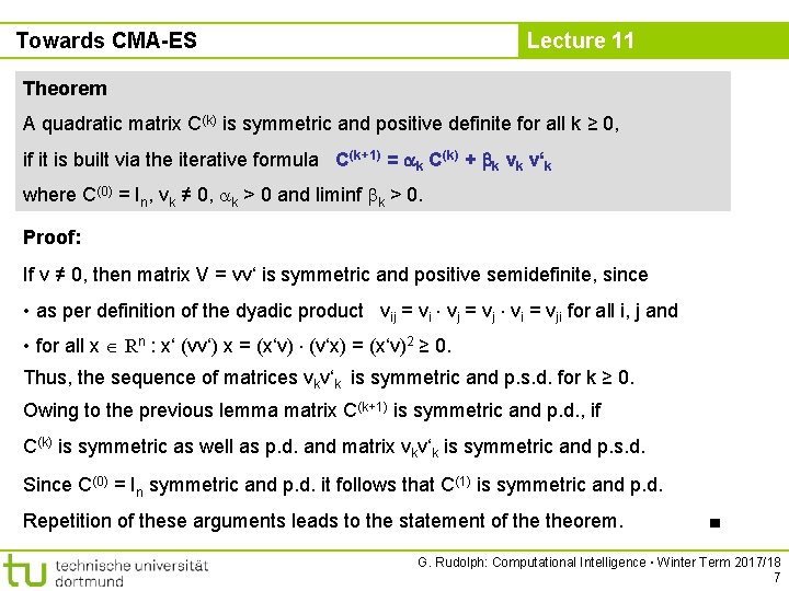
Towards CMA-ES Lecture 11 Theorem A quadratic matrix C(k) is symmetric and positive definite for all k ≥ 0, if it is built via the iterative formula C(k+1) = k C(k) + k vk v‘k where C(0) = In, vk ≠ 0, k > 0 and liminf k > 0. Proof: If v ≠ 0, then matrix V = vv‘ is symmetric and positive semidefinite, since • as per definition of the dyadic product vij = vi vj = vj vi = vji for all i, j and • for all x Rn : x‘ (vv‘) x = (x‘v) (v‘x) = (x‘v)2 ≥ 0. Thus, the sequence of matrices vkv‘k is symmetric and p. s. d. for k ≥ 0. Owing to the previous lemma matrix C(k+1) is symmetric and p. d. , if C(k) is symmetric as well as p. d. and matrix vkv‘k is symmetric and p. s. d. Since C(0) = In symmetric and p. d. it follows that C(1) is symmetric and p. d. Repetition of these arguments leads to the statement of theorem. ■ G. Rudolph: Computational Intelligence ▪ Winter Term 2017/18 7

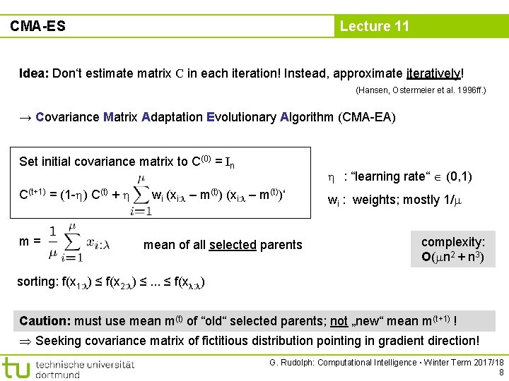
CMA-ES Lecture 11 Idea: Don‘t estimate matrix C in each iteration! Instead, approximate iteratively! (Hansen, Ostermeier et al. 1996 ff. ) → Covariance Matrix Adaptation Evolutionary Algorithm (CMA-EA) Set initial covariance matrix to C(0) = In C(t+1) = (1 - ) C(t) + m= : “learning rate“ (0, 1) wi (xi: – m(t))‘ mean of all selected parents wi : weights; mostly 1/ complexity: O( n 2 + n 3) sorting: f(x 1: ) ≤ f(x 2: ) ≤. . . ≤ f(x : ) Caution: must use mean m(t) of “old“ selected parents; not „new“ mean m(t+1) ! Seeking covariance matrix of fictitious distribution pointing in gradient direction! G. Rudolph: Computational Intelligence ▪ Winter Term 2017/18 8

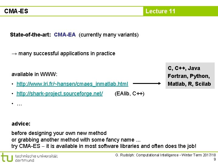
CMA-ES Lecture 11 State-of-the-art: CMA-EA (currently many variants) → many successful applications in practice available in WWW: • http: //www. lri. fr/~hansen/cmaes_inmatlab. html • http: //shark-project. sourceforge. net/ C, C++, Java Fortran, Python, Matlab, R, Scilab (EAlib, C++) • … advice: before designing your own new method or grabbing another method with some fancy name. . . try CMA-ES it is available in most software libraries and often does the job! G. Rudolph: Computational Intelligence ▪ Winter Term 2017/18 9