Computational Intelligence Winter Term 201314 Prof Dr Gnter

Computational Intelligence Winter Term 2013/14 Prof. Dr. Günter Rudolph Lehrstuhl für Algorithm Engineering (LS 11) Fakultät für Informatik TU Dortmund

Plan for Today Lecture 03 ● Application Fields of ANNs § Classification § Prediction § Function Approximation ● Radial Basis Function Nets (RBF Nets) § Model § Training ● Recurrent MLP § Elman Nets § Jordan Nets G. Rudolph: Computational Intelligence ▪ Winter Term 2013/14 2

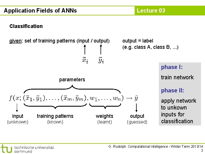
Application Fields of ANNs Lecture 03 Classification given: set of training patterns (input / output) output = label (e. g. class A, class B, . . . ) phase I: train network parameters phase II: input training patterns weights output (unknown) (learnt) (guessed) apply network to unkown inputs for classification G. Rudolph: Computational Intelligence ▪ Winter Term 2013/14 3

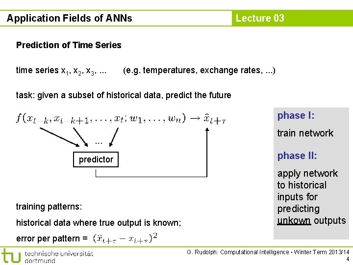
Application Fields of ANNs Lecture 03 Prediction of Time Series time series x 1, x 2, x 3, . . . (e. g. temperatures, exchange rates, . . . ) task: given a subset of historical data, predict the future phase I: . . . predictor training patterns: historical data where true output is known; train network phase II: apply network to historical inputs for predicting unkown outputs error per pattern = G. Rudolph: Computational Intelligence ▪ Winter Term 2013/14 4

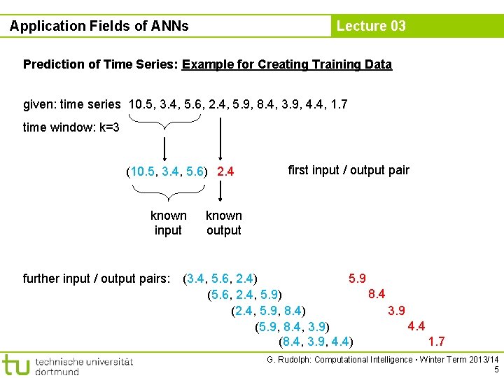
Application Fields of ANNs Lecture 03 Prediction of Time Series: Example for Creating Training Data given: time series 10. 5, 3. 4, 5. 6, 2. 4, 5. 9, 8. 4, 3. 9, 4. 4, 1. 7 time window: k=3 (10. 5, 3. 4, 5. 6) 2. 4 known input further input / output pairs: first input / output pair known output (3. 4, 5. 6, 2. 4) 5. 9 8. 4 (5. 6, 2. 4, 5. 9) (2. 4, 5. 9, 8. 4) 3. 9 4. 4 (5. 9, 8. 4, 3. 9) (8. 4, 3. 9, 4. 4) 1. 7 G. Rudolph: Computational Intelligence ▪ Winter Term 2013/14 5

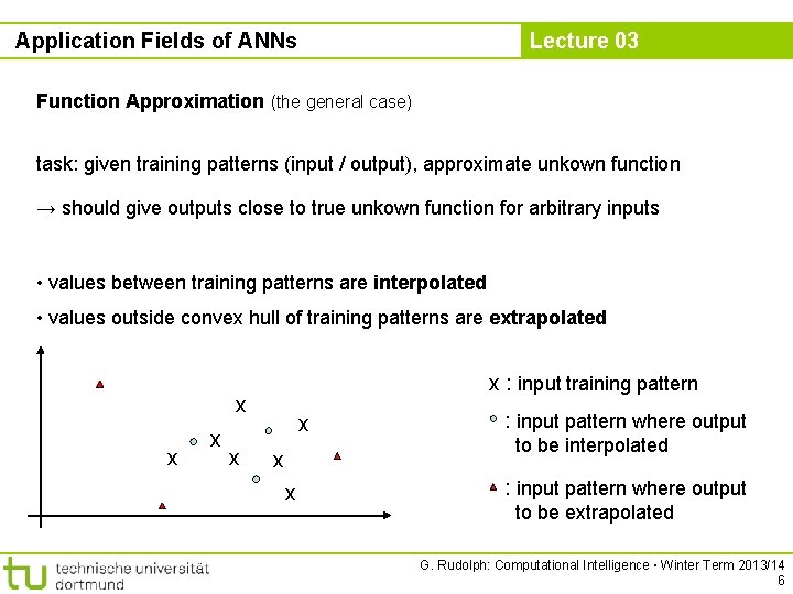
Application Fields of ANNs Lecture 03 Function Approximation (the general case) task: given training patterns (input / output), approximate unkown function → should give outputs close to true unkown function for arbitrary inputs • values between training patterns are interpolated • values outside convex hull of training patterns are extrapolated x : input training pattern x x x x : input pattern where output to be interpolated : input pattern where output to be extrapolated G. Rudolph: Computational Intelligence ▪ Winter Term 2013/14 6

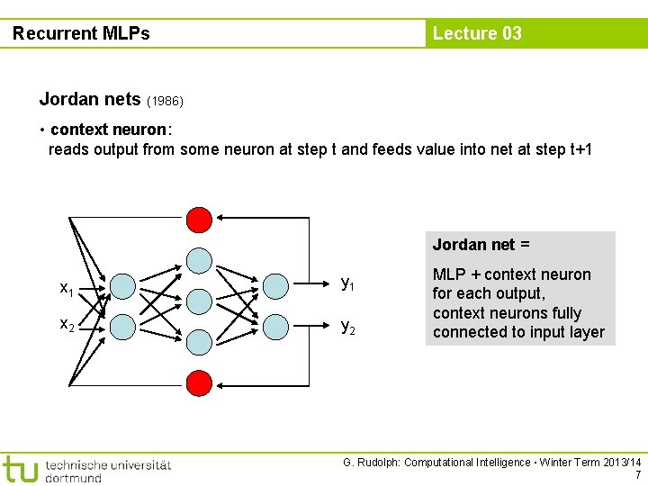
Recurrent MLPs Lecture 03 Jordan nets (1986) • context neuron: reads output from some neuron at step t and feeds value into net at step t+1 Jordan net = x 1 y 1 x 2 y 2 MLP + context neuron for each output, context neurons fully connected to input layer G. Rudolph: Computational Intelligence ▪ Winter Term 2013/14 7

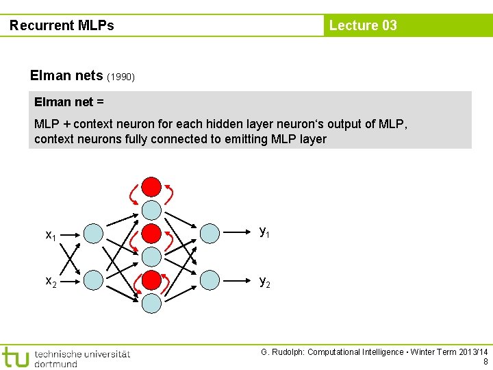
Recurrent MLPs Lecture 03 Elman nets (1990) Elman net = MLP + context neuron for each hidden layer neuron‘s output of MLP, context neurons fully connected to emitting MLP layer x 1 y 1 x 2 y 2 G. Rudolph: Computational Intelligence ▪ Winter Term 2013/14 8

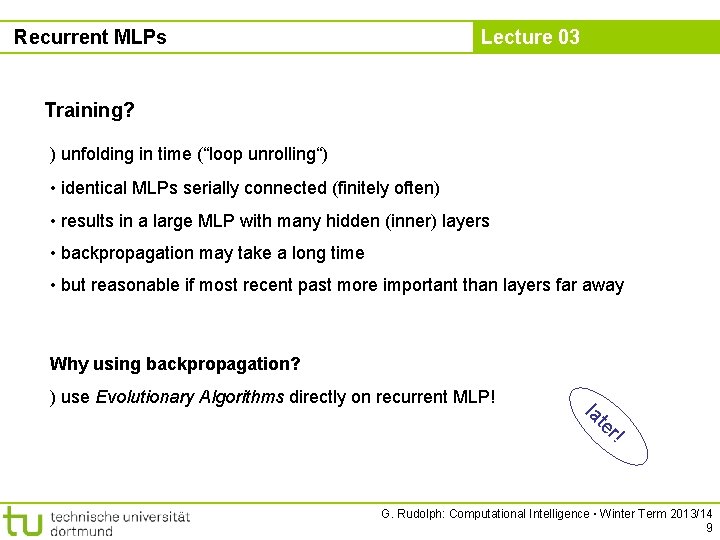
Recurrent MLPs Lecture 03 Training? ) unfolding in time (“loop unrolling“) • identical MLPs serially connected (finitely often) • results in a large MLP with many hidden (inner) layers • backpropagation may take a long time • but reasonable if most recent past more important than layers far away Why using backpropagation? ) use Evolutionary Algorithms directly on recurrent MLP! la te r! G. Rudolph: Computational Intelligence ▪ Winter Term 2013/14 9

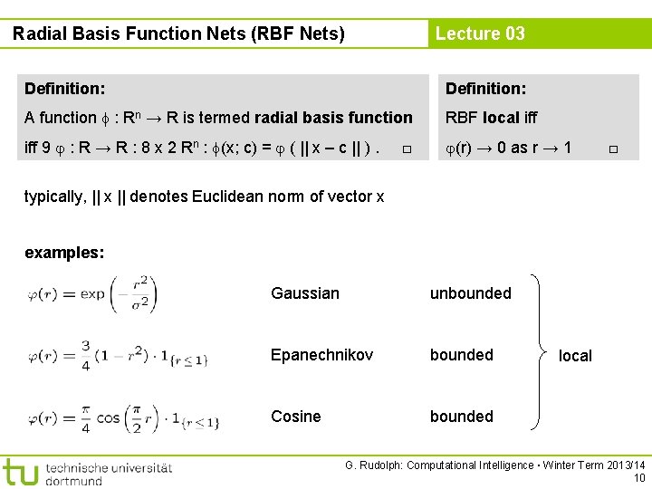
Radial Basis Function Nets (RBF Nets) Lecture 03 Definition: A function : Rn → R is termed radial basis function RBF local iff 9 : R → R : 8 x 2 Rn : (x; c) = ( || x – c || ). (r) → 0 as r → 1 □ □ typically, || x || denotes Euclidean norm of vector x examples: Gaussian unbounded Epanechnikov bounded Cosine bounded local G. Rudolph: Computational Intelligence ▪ Winter Term 2013/14 10

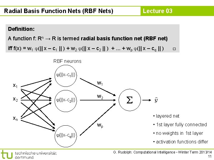
Radial Basis Function Nets (RBF Nets) Lecture 03 Definition: A function f: Rn → R is termed radial basis function net (RBF net) iff f(x) = w 1 (|| x – c 1 || ) + w 2 (|| x – c 2 || ) +. . . + wp (|| x – cq || ) □ RBF neurons (||x-c 1||) w 1 x 2 (||x-c 2||) w 2 • layered net xn wp (||x-cq||) • 1 st layer fully connected • no weights in 1 st layer • activation functions differ G. Rudolph: Computational Intelligence ▪ Winter Term 2013/14 11

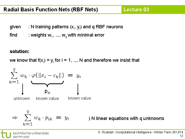
Radial Basis Function Nets (RBF Nets) Lecture 03 given : N training patterns (xi, yi) and q RBF neurons find : weights w 1, . . . , wq with minimal error solution: we know that f(xi) = yi for i = 1, . . . , N and therefore we insist that pik unknown value ) N linear equations with q unknowns G. Rudolph: Computational Intelligence ▪ Winter Term 2013/14 12

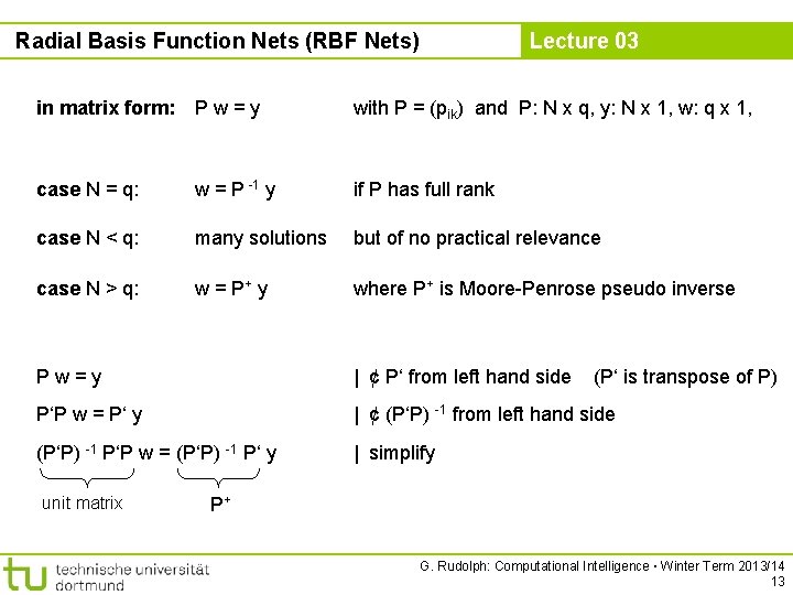
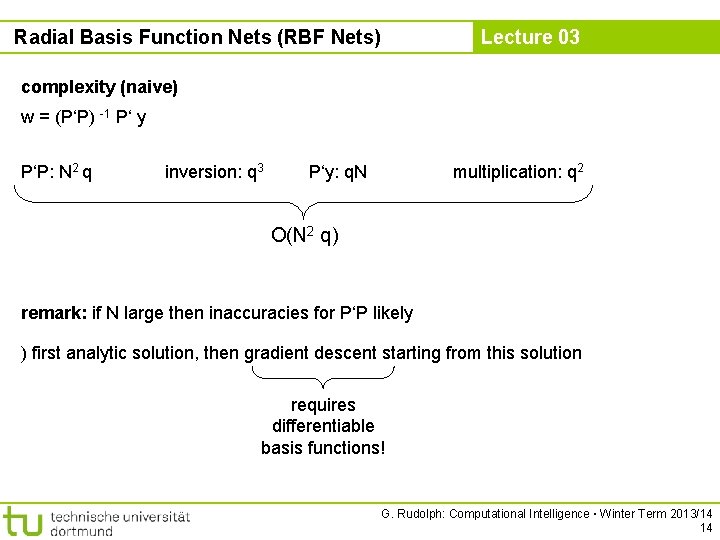
Radial Basis Function Nets (RBF Nets) Lecture 03 in matrix form: Pw=y with P = (pik) and P: N x q, y: N x 1, w: q x 1, case N = q: w = P -1 y if P has full rank case N < q: many solutions but of no practical relevance case N > q: w = P+ y where P+ is Moore-Penrose pseudo inverse Pw=y | ¢ P‘ from left hand side P‘P w = P‘ y | ¢ (P‘P) -1 from left hand side (P‘P) -1 P‘P w = (P‘P) -1 P‘ y | simplify unit matrix (P‘ is transpose of P) P+ G. Rudolph: Computational Intelligence ▪ Winter Term 2013/14 13

Radial Basis Function Nets (RBF Nets) Lecture 03 complexity (naive) w = (P‘P) -1 P‘ y P‘P: N 2 q inversion: q 3 P‘y: q. N multiplication: q 2 O(N 2 q) remark: if N large then inaccuracies for P‘P likely ) first analytic solution, then gradient descent starting from this solution requires differentiable basis functions! G. Rudolph: Computational Intelligence ▪ Winter Term 2013/14 14

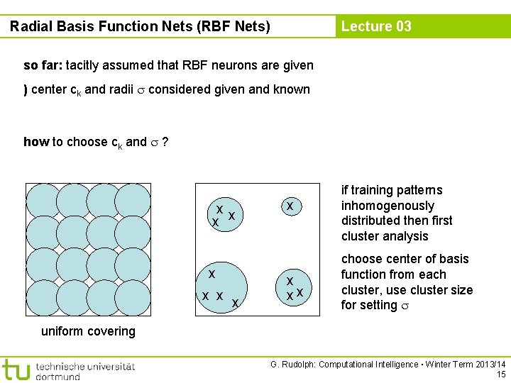
Radial Basis Function Nets (RBF Nets) Lecture 03 so far: tacitly assumed that RBF neurons are given ) center ck and radii considered given and known how to choose ck and ? xx x x x xx if training patterns inhomogenously distributed then first cluster analysis choose center of basis function from each cluster, use cluster size for setting uniform covering G. Rudolph: Computational Intelligence ▪ Winter Term 2013/14 15

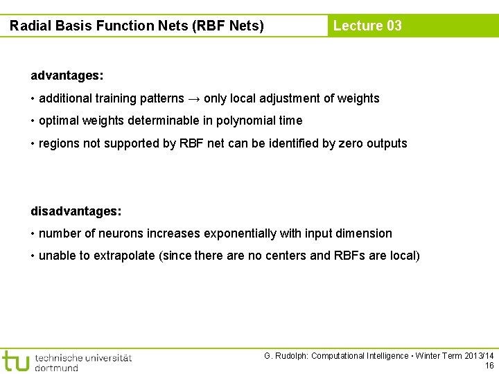
Radial Basis Function Nets (RBF Nets) Lecture 03 advantages: • additional training patterns → only local adjustment of weights • optimal weights determinable in polynomial time • regions not supported by RBF net can be identified by zero outputs disadvantages: • number of neurons increases exponentially with input dimension • unable to extrapolate (since there are no centers and RBFs are local) G. Rudolph: Computational Intelligence ▪ Winter Term 2013/14 16