Computational Intelligence Methods and Applications Lecture 30 Neurofuzzy

Computational Intelligence: Methods and Applications Lecture 30 Neurofuzzy system FSM and covering algorithms. Włodzisław Duch Dept. of Informatics, UMK Google: W Duch

Training FSM network Parameters of the network nodes may be estimated using maximum likelihood Expectation Maximization learning. Computationally simpler iterative schemes have been proposed. An outline of the FSM (Feature Space Mapping) separable function network algorithm implemented in Ghost. Miner: • Select the type of functions and desired accuracy. • Initialize network parameters: find main clusters, their centers and dispersions; include cluster rotations. • Adaptation phase: read the training data, if error is made adapt the parameters of the network to reduce them - move the closest centers towards the data, increase dispersions. • Growth phase: if accuracy cannot be improved further add new nodes (functions) in areas where most errors occur. • Cleaning phase: remove functions with smallest coverage, retrain.

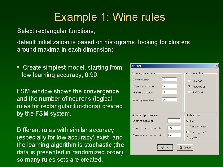
Example 1: Wine rules Select rectangular functions; default initialization is based on histograms, looking for clusters around maxima in each dimension; • Create simplest model, starting from low learning accuracy, 0. 90. FSM window shows the convergence and the number of neurons (logical rules for rectangular functions) created by the FSM system. Different rules with similar accuracy (especially for low accuracy) exist, and the learning algorithm is stochastic (the data is presented in randomized order), so many rules sets are created.

Experiments with Wine rules Run FSM with different parameters and note how different set of rules are generated. FSM may discover new, simple rules, that trees will not find, for ex: if proline > 929. 5 then class 1 (48 covered, 3 errors, but 2 corrected by other rules). if color < 3. 792 then class 2 (63 cases, 60 correct, 3 errors) Trees generate hierarchical path; FSM covers the data samples with rectangular functions, minimizing the number of features used. FSM includes stochastic learning (samples are randomized). Weak: large variance for high accuracy models. Strong: many simple models may be generated, experts may like some more than the others.

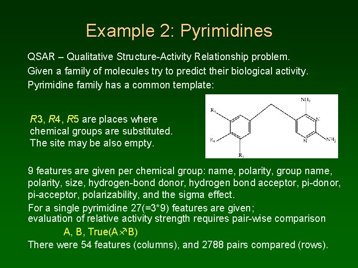
Example 2: Pyrimidines QSAR – Qualitative Structure-Activity Relationship problem. Given a family of molecules try to predict their biological activity. Pyrimidine family has a common template: R 3, R 4, R 5 are places where chemical groups are substituted. The site may be also empty. 9 features are given per chemical group: name, polarity, group name, polarity, size, hydrogen-bond donor, hydrogen bond acceptor, pi-donor, pi-acceptor, polarizability, and the sigma effect. For a single pyrimidine 27(=3*9) features are given; evaluation of relative activity strength requires pair-wise comparison A, B, True(A B) There were 54 features (columns), and 2788 pairs compared (rows).

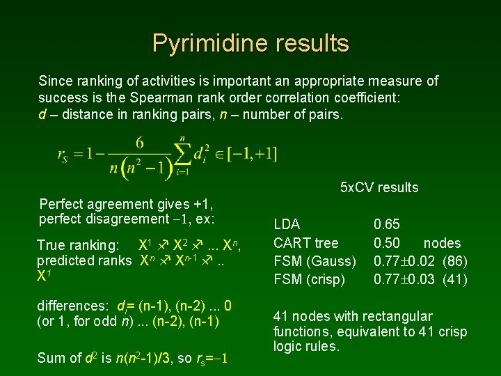
Pyrimidine results Since ranking of activities is important an appropriate measure of success is the Spearman rank order correlation coefficient: d – distance in ranking pairs, n – number of pairs. 5 x. CV results Perfect agreement gives +1, perfect disagreement -1, ex: True ranking: X 1 X 2 . . . Xn, predicted ranks Xn Xn-1 . . X 1 differences: di= (n-1), (n-2). . . 0 (or 1, for odd n). . . (n-2), (n-1) Sum of d 2 is n(n 2 -1)/3, so rs=-1 LDA CART tree FSM (Gauss) FSM (crisp) 0. 65 0. 50 nodes 0. 77 0. 02 (86) 0. 77 0. 03 (41) 41 nodes with rectangular functions, equivalent to 41 crisp logic rules.

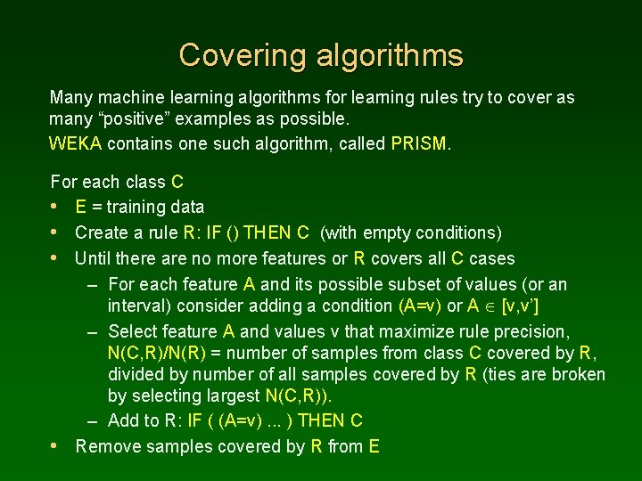
Covering algorithms Many machine learning algorithms for learning rules try to cover as many “positive” examples as possible. WEKA contains one such algorithm, called PRISM. For each class C • E = training data • Create a rule R: IF () THEN C (with empty conditions) • Until there are no more features or R covers all C cases – For each feature A and its possible subset of values (or an interval) consider adding a condition (A=v) or A [v, v’] – Select feature A and values v that maximize rule precision, N(C, R)/N(R) = number of samples from class C covered by R, divided by number of all samples covered by R (ties are broken by selecting largest N(C, R)). – Add to R: IF ( (A=v). . . ) THEN C • Remove samples covered by R from E

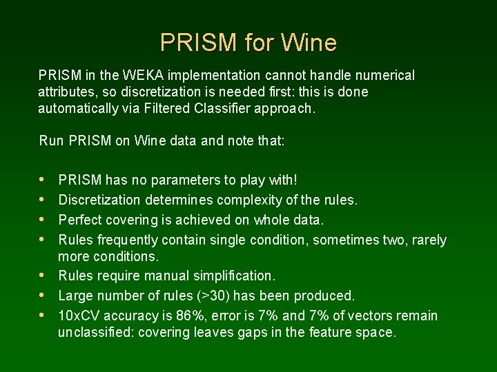
PRISM for Wine PRISM in the WEKA implementation cannot handle numerical attributes, so discretization is needed first: this is done automatically via Filtered Classifier approach. Run PRISM on Wine data and note that: • • PRISM has no parameters to play with! Discretization determines complexity of the rules. Perfect covering is achieved on whole data. Rules frequently contain single condition, sometimes two, rarely more conditions. • Rules require manual simplification. • Large number of rules (>30) has been produced. • 10 x. CV accuracy is 86%, error is 7% and 7% of vectors remain unclassified: covering leaves gaps in the feature space.