Computational Intelligence Methods and Applications Lecture 18 Decision

Computational Intelligence: Methods and Applications Lecture 18 Decision trees Włodzisław Duch Dept. of Informatics, UMK Google: W Duch

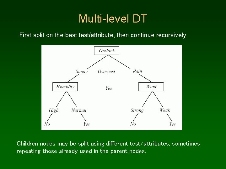
Multi-level DT First split on the best test/attribute, then continue recursively. Children nodes may be split using different test/attributes, sometimes repeating those already used in the parent nodes.

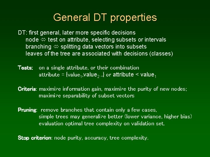
General DT properties DT: first general, later more specific decisions node test on attribute, selecting subsets or intervals branching splitting data vectors into subsets leaves of the tree are associated with decisions (classes) Tests: on a single attribute, or their combination attribute = {value 1, value 2. . } or attribute < value 1 Criteria: maximize information gain, maximize the purity of new nodes; maximize separability of subset vectors Pruning: remove branches that contain only a few cases, simple trees may generalize better (lower variance, higher bias) evaluation optimal tree complexity on validation set. Stop criterion: node purity, accuracy, tree complexity.

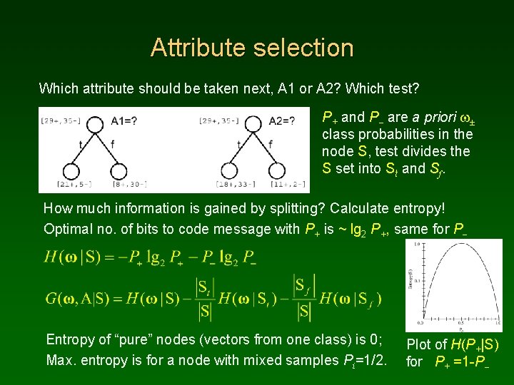
Attribute selection Which attribute should be taken next, A 1 or A 2? Which test? P+ and P- are a priori w± class probabilities in the node S, test divides the S set into St and Sf. How much information is gained by splitting? Calculate entropy! Optimal no. of bits to code message with P+ is ~ lg 2 P+, same for P- Entropy of “pure” nodes (vectors from one class) is 0; Max. entropy is for a node with mixed samples Pi=1/2. Plot of H(P+|S) for P+ =1 -P-

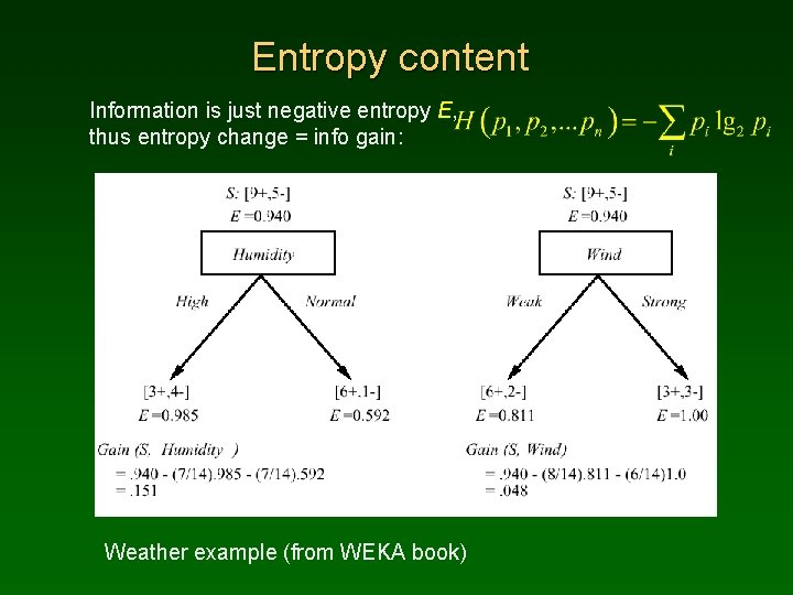
Entropy content Information is just negative entropy E, thus entropy change = info gain: Weather example (from WEKA book)

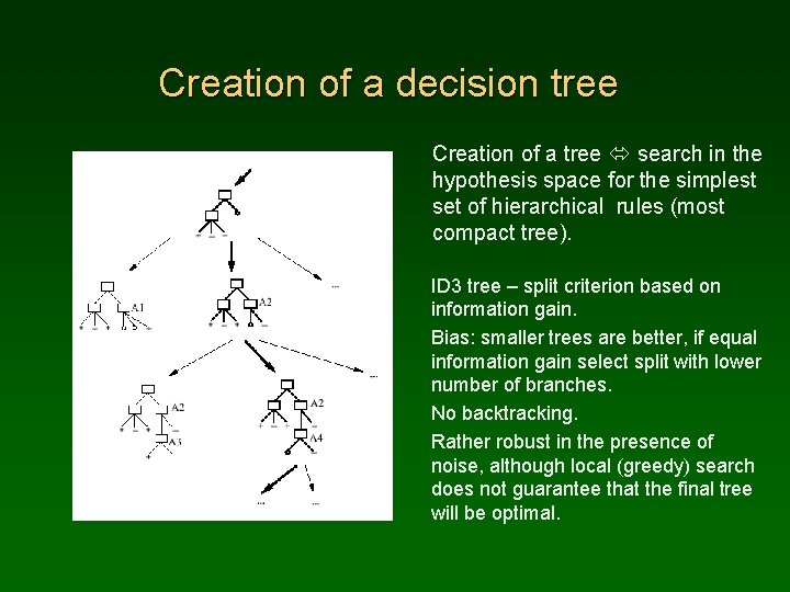
Creation of a decision tree Creation of a tree search in the hypothesis space for the simplest set of hierarchical rules (most compact tree). ID 3 tree – split criterion based on information gain. Bias: smaller trees are better, if equal information gain select split with lower number of branches. No backtracking. Rather robust in the presence of noise, although local (greedy) search does not guarantee that the final tree will be optimal.

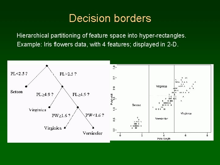
Decision borders Hierarchical partitioning of feature space into hyper-rectangles. Example: Iris flowers data, with 4 features; displayed in 2 -D.

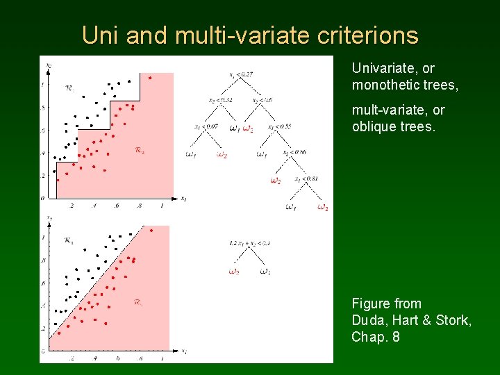
Uni and multi-variate criterions Univariate, or monothetic trees, mult-variate, or oblique trees. Figure from Duda, Hart & Stork, Chap. 8

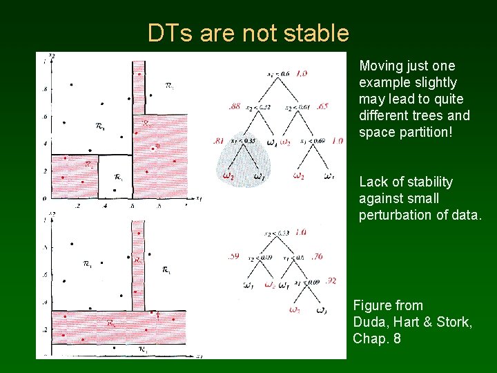
DTs are not stable Moving just one example slightly may lead to quite different trees and space partition! Lack of stability against small perturbation of data. Figure from Duda, Hart & Stork, Chap. 8

Ockham’s razor Why simple trees should be preferred? 1. 2. 3. The number of simple hypothesis that may accidentally fit the data is small, so chances that simple hypothesis uncover some interesting knowledge about the data are larger. Simpler trees have higher bias and thus lower variance, they should not overfit the data that easily. Simpler trees do not partition the feature space into too many small boxes and may generalize better; complex trees may create a separate box for each training data sample. Still, even if the tree is small. . . sufficiently long search by pure chance may find false solution; for small datasets with many attributes several equivalent (from the accuracy point of view) descriptions may exist. => One tree is not sufficient, we need a forest of healthy trees!

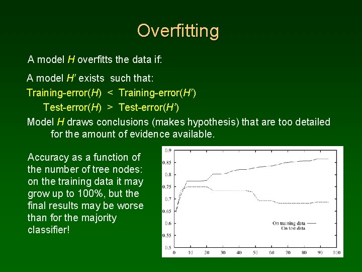
Overfitting A model H overfitts the data if: A model H’ exists such that: Training-error(H) < Training-error(H’) Test-error(H) > Test-error(H’) Model H draws conclusions (makes hypothesis) that are too detailed for the amount of evidence available. Accuracy as a function of the number of tree nodes: on the training data it may grow up to 100%, but the final results may be worse than for the majority classifier!

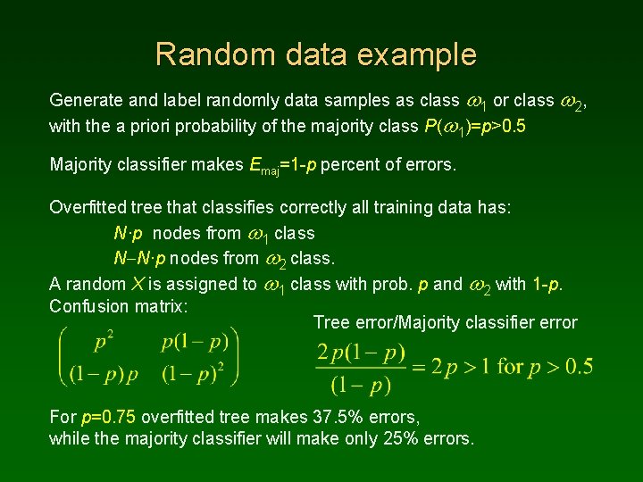
Random data example Generate and label randomly data samples as class w 1 or class w 2, with the a priori probability of the majority class P(w 1)=p>0. 5 Majority classifier makes Emaj=1 -p percent of errors. Overfitted tree that classifies correctly all training data has: N·p nodes from w 1 class N-N·p nodes from w 2 class. A random X is assigned to w 1 class with prob. p and w 2 with 1 -p. Confusion matrix: Tree error/Majority classifier error For p=0. 75 overfitted tree makes 37. 5% errors, while the majority classifier will make only 25% errors.

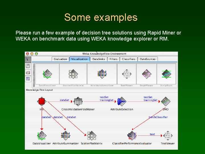
Some examples Please run a few example of decision tree solutions using Rapid Miner or WEKA on benchmark data using WEKA knowledge explorer or RM.