Computational Complexity Theory Lecture 1 Intro Turing machines

Computational Complexity Theory Lecture 1: Intro; Turing machines Indian Institute of Science

About the course �Computational complexity attempts to classify computational problems based on the amount of resources required by algorithms to solve them.

About the course �Computational complexity attempts to classify computational problems based on the amount of resources required by algorithms to solve them. �Computational problems come in various flavors:

About the course �Computational complexity attempts to classify computational problems based on the amount of resources required by algorithms to solve them. �Computational problems come in various flavors: a. Decision problem Example: Is vertex t reachable from vertex s in graph G? (…output is YES/NO)

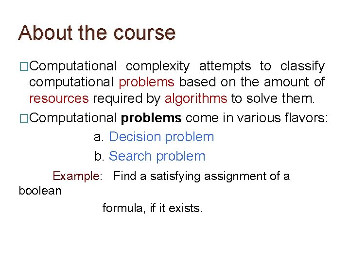
About the course �Computational complexity attempts to classify computational problems based on the amount of resources required by algorithms to solve them. �Computational problems come in various flavors: a. Decision problem b. Search problem Example: Find a satisfying assignment of a boolean formula, if it exists.

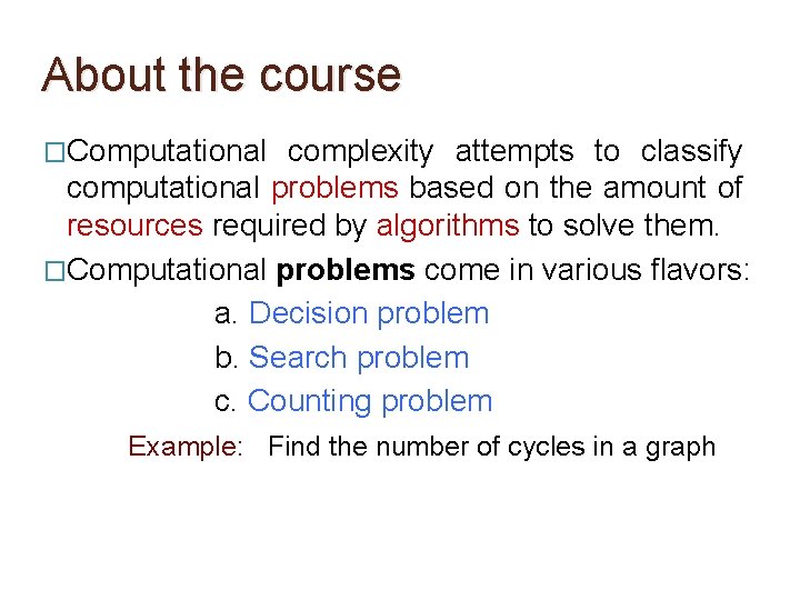
About the course �Computational complexity attempts to classify computational problems based on the amount of resources required by algorithms to solve them. �Computational problems come in various flavors: a. Decision problem b. Search problem c. Counting problem Example: Find the number of cycles in a graph

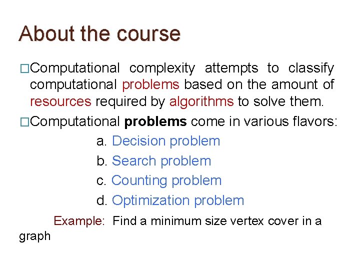
About the course �Computational complexity attempts to classify computational problems based on the amount of resources required by algorithms to solve them. �Computational problems come in various flavors: a. Decision problem b. Search problem c. Counting problem d. Optimization problem Example: Find a minimum size vertex cover in a graph

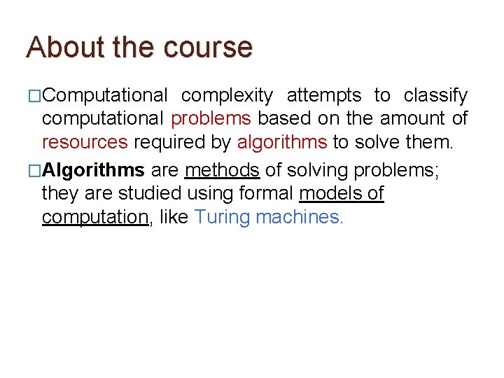
About the course �Computational complexity attempts to classify computational problems based on the amount of resources required by algorithms to solve them. �Algorithms are methods of solving problems; they are studied using formal models of computation, like Turing machines.

About the course �Computational complexity attempts to classify computational problems based on the amount of resources required by algorithms to solve them. �Algorithms are methods of solving problems; they are studied using formal models of computation, like Turing machines. • a memory with head (like a RAM)

About the course �Computational complexity attempts to classify computational problems based on the amount of resources required by algorithms to solve them. �Algorithms are methods of solving problems; they are studied using formal models of computation, like Turing machines. • a memory with head (like a RAM) • a finite control (like a processor)

About the course �Computational complexity attempts to classify computational problems based on the amount of resources required by algorithms to solve them. �Algorithms are methods of solving problems; they are studied using formal models of computation, like Turing machines. (…more later)

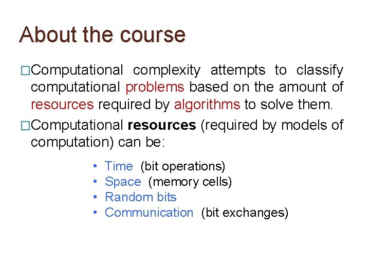
About the course �Computational complexity attempts to classify computational problems based on the amount of resources required by algorithms to solve them. �Computational resources (required by models of computation) can be: • Time (bit operations) • Space (memory cells)

About the course �Computational complexity attempts to classify computational problems based on the amount of resources required by algorithms to solve them. �Computational resources (required by models of computation) can be: • • Time (bit operations) Space (memory cells) Random bits Communication (bit exchanges)

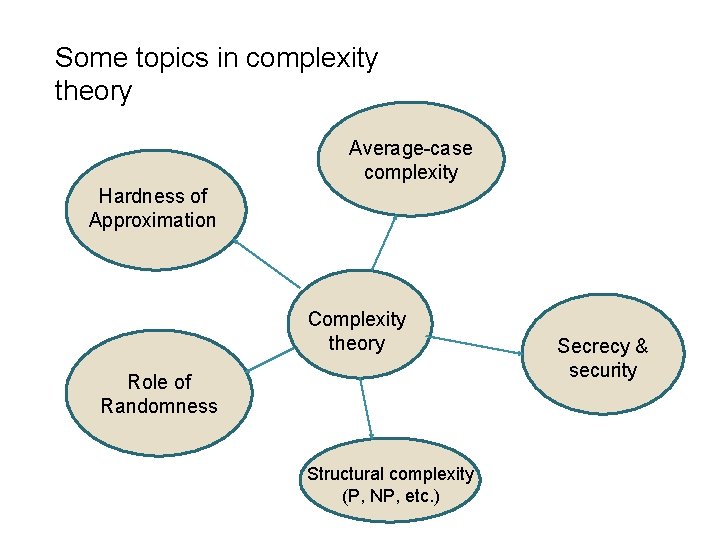
Some topics in complexity theory Average-case complexity Hardness of Approximation Complexity theory Role of Randomness Structural complexity (P, NP, etc. ) Secrecy & security

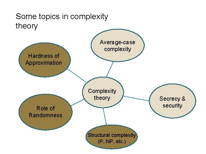
Some topics in complexity theory Average-case complexity Hardness of Approximation Complexity theory Role of Randomness Structural complexity (P, NP, etc. ) Secrecy & security

Structural Complexity �Classes P, NP, co-NP… NP-completeness.

Structural Complexity �Classes P, NP, co-NP… NP-completeness. How hard is it to check satisfiability of a boolean formula that has exactly one or no satisfying assignment?

Structural Complexity �Classes P, NP, co-NP… NP-completeness. �Space bounded computation.

Structural Complexity �Classes P, NP, co-NP… NP-completeness. �Space bounded computation. How much space is required to check s-t connectivity?

Structural Complexity �Classes P, NP, co-NP… NP-completeness. �Space bounded computation. �Counting complexity.

Structural Complexity �Classes P, NP, co-NP… NP-completeness. �Space bounded computation. �Counting complexity. How hard is it to count the number of perfect matchings in a graph?

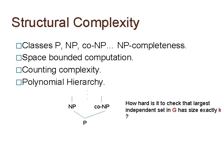
Structural Complexity �Classes P, NP, co-NP… NP-completeness. �Space bounded computation. �Counting complexity. �Polynomial Hierarchy. . NP co-NP P How hard is it to check that largest independent set in G has size exactly k ?

Structural Complexity �Classes P, NP, co-NP… NP-completeness. �Space bounded computation. �Counting complexity. �Polynomial Hierarchy. How hard is it to find a minimum size circuit computing the same boolean function as a given boolean circuit?

Structural Complexity �Classes P, NP, co-NP… NP-completeness. �Space bounded computation. �Counting complexity. �Polynomial Hierarchy. �Boolean circuits and circuit lower bounds.

Structural Complexity �Classes P, NP, co-NP… NP-completeness. �Space bounded computation. �Counting complexity. �Polynomial Hierarchy. �Boolean circuits and circuit lower bounds. A central topic in classical complecity theory; Proving P≠NP reduces to showing circuit lower bounds.

Role of Randomness in Computation �Probabilistic complexity classes.

Role of Randomness in Computation �Probabilistic complexity classes. • Does randomization help in improving efficiency? • Quicksort has O(n log n) expected time but O(n^2) worst case time. • Can SAT be solved in polynomial time using randomness? Theorem (Schoening, 1999): 3 SAT can be solved in randomized O((4/3)n) time.

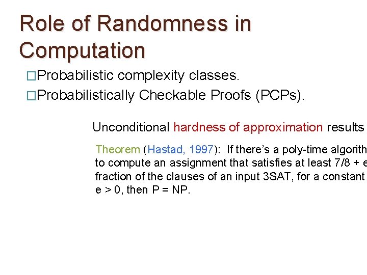
Role of Randomness in Computation �Probabilistic complexity classes. �Probabilistically Checkable Proofs (PCPs).

Role of Randomness in Computation �Probabilistic complexity classes. �Probabilistically Checkable Proofs (PCPs). Unconditional hardness of approximation results Theorem (Hastad, 1997): If there’s a poly-time algorith to compute an assignment that satisfies at least 7/8 + e fraction of the clauses of an input 3 SAT, for a constant e > 0, then P = NP.

Role of Randomness in Computation �Probabilistic complexity classes. �Probabilistically Checkable Proofs (PCPs). �A glimpse of pseudorandom generators (if time permits).

Role of Randomness in Computation �Probabilistic complexity classes. �Probabilistically Checkable Proofs (PCPs). �A glimpse of pseudorandom generators (if time permits). Can every polynomial-time randomized algorithm be derandomized to a deterministic polynomial-time algorithm?

Average-case Complexity �Distributional problems. How hard is it to solve the clique problem on inputs chosen from a “real-life” distribution?

Average-case Complexity �Distributional problems. �Hardness amplification: From weak to strong hardness. In cryptographic applications, we need hard on average functions for secure encryptions.

Basic Course Info �Course title: Computational Complexity Theory �Credits: 3: 1 Instructor: Chandan Saha �Class timings : Monday, Wednesday: 3: 30 -5 pm. �Venue: CSA lecture hall 117. �Primary reference: Computational Complexity – A Modern Approach by Sanjeev Arora and Boaz Barak.

Basic Course Info � Prerequisites � Grading : Basic familiarity with algorithms; Some mathematical maturity will be helpful. policy : Assignments - 30% Mid-term - 35% End-term - 35% Course homepage: drona. csa. iisc. ac. in/~chandan/courses/complexity 18/home. html

Let’s begin…

Turing Machines �An algorithm is a set of instructions or rules. �To understand the performance of an algorithm we need a model of computation. Turing machine is one such natural model.

Turing Machines �An algorithm is a set of instructions or rules. �To understand the performance of an algorithm we need a model of computation. Turing machine is one such natural model. �A TM consists of: • Memory tape(s) • A finite set of rules

Turing Machines �An algorithm is a set of instructions or rules. �To understand the performance of an algorithm we need a model of computation. Turing machine is one such natural model. �A TM consists of: • Memory tape(s) • A finite set of rules �Turing machines A mathematical way to describe algorithms.

Turing Machines �An algorithm is a set of instructions or rules. �To understand the performance of an algorithm we need a model of computation. Turing machine is one such natural model. �A TM consists of: • Memory tape(s) • A finite set of rules (e. g. of a physical realization a TM is a simple adder)

Turing Machines �Definition. A k-tape Turing Machine M is described by a tuple (Γ, Q, δ) such that

Turing Machines �Definition. A k-tape Turing Machine M is described by a tuple (Γ, Q, δ) such that �M has k memory tapes (input/work/output tapes) with heads; �Γis a finite set of alphabets. (Every memory cell contains an element of Γ)

Turing Machines �Definition. A k-tape Turing Machine M is described by a tuple (Γ, Q, δ) such that �M has k memory tapes (input/work/output tapes) with heads; �Γis a finite set of alphabets. (Every memory cell contains an element of Γ) has a blank symbol

Turing Machines �Definition. A k-tape Turing Machine M is described by a tuple (Γ, Q, δ) such that �M has k memory tapes (input/work/output tapes) with heads; �Γis a finite set of alphabets. (Every memory cell contains an element of Γ) �Q is a finite set of states. (special states: qstart , k k k qhalt) �δ is a function from Q x Γ to Q x Γ x {L, S, R}

Turing Machines �Definition. A k-tape Turing Machine M is described by a tuple (Γ, Q, δ) such that �M has k memory tapes (input/work/output tapes) with heads; �Γis a finite set of alphabets. (Every memory cell contains an element of Γ) �Q is a finite set of states. (special states: qstart , k k k qhalt) �δ is a function from Q x Γ to Q x Γ x {L, S, R} known as transition function; it captures the dynamics of M

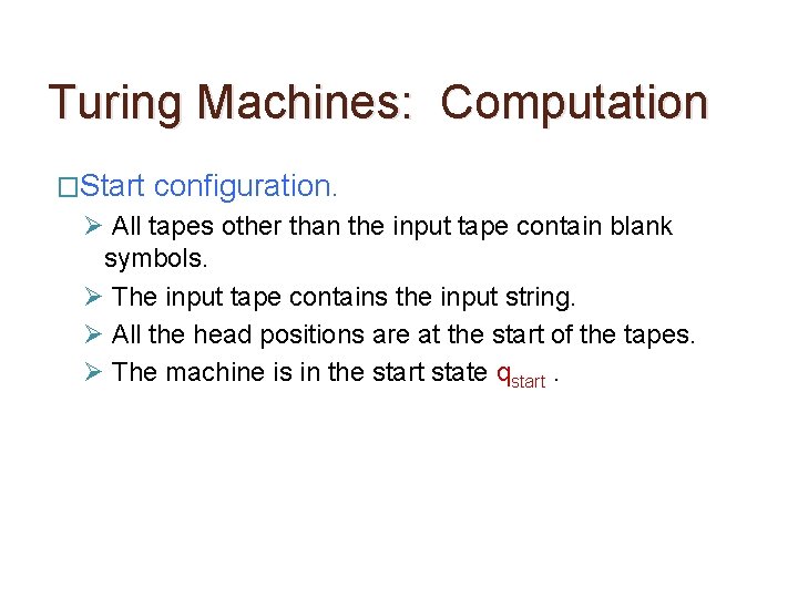
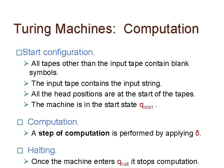
Turing Machines: Computation �Start configuration. Ø All tapes other than the input tape contain blank symbols. Ø The input tape contains the input string. Ø All the head positions are at the start of the tapes. Ø The machine is in the start state qstart.

Turing Machines: Computation �Start configuration. Ø All tapes other than the input tape contain blank symbols. Ø The input tape contains the input string. Ø All the head positions are at the start of the tapes. Ø The machine is in the start state qstart. � Computation. Ø A step of computation is performed by applying δ. � Halting. Ø Once the machine enters qhalt it stops computation.

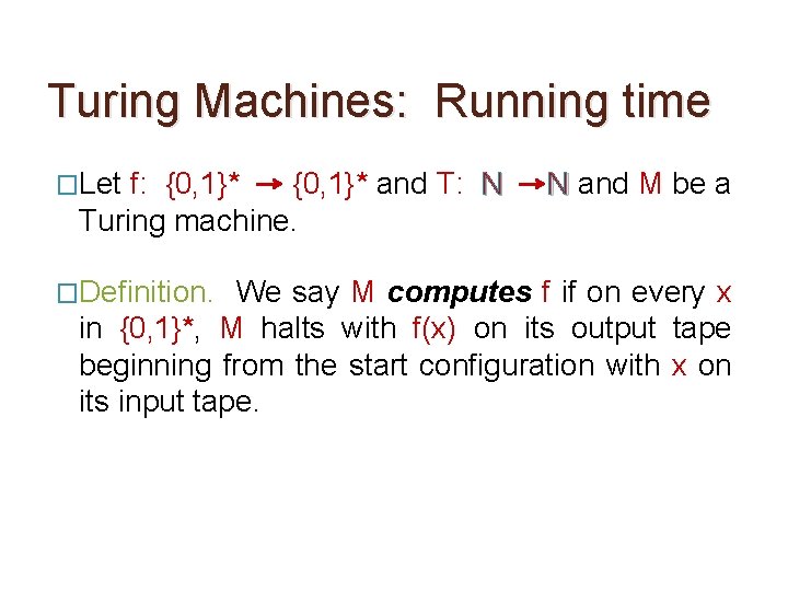
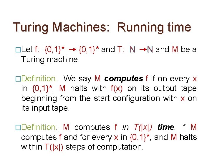
Turing Machines: Running time �Let f: {0, 1}* and T: N Turing machine. �Definition. N and M be a We say M computes f if on every x in {0, 1}*, M halts with f(x) on its output tape beginning from the start configuration with x on its input tape.

Turing Machines: Running time �Let f: {0, 1}* and T: N Turing machine. N and M be a �Definition. We say M computes f if on every x in {0, 1}*, M halts with f(x) on its output tape beginning from the start configuration with x on its input tape. �Definition. M computes f in T(|x|) time, if M computes f and for every x in {0, 1}*, and M halts within T(|x|) steps of computation.

Turing Machines �In this course, we would be dealing with Ø Turing machines that halt on every input. Ø Computational problems that can be solved by Turing machines.

Turing Machines �In this course, we would be dealing with Ø Turing machines that halt on every input. Ø Computational problems that can be solved by Turing machines. � Can every computational problem be solved using Turing machines?

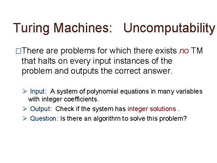
Turing Machines: Uncomputability �There are problems for which there exists no TM that halts on every input instances of the problem and outputs the correct answer. Ø Input: A system of polynomial equations in many variables with integer coefficients. Ø Output: Check if the system has integer solutions. Ø Question: Is there an algorithm to solve this problem?

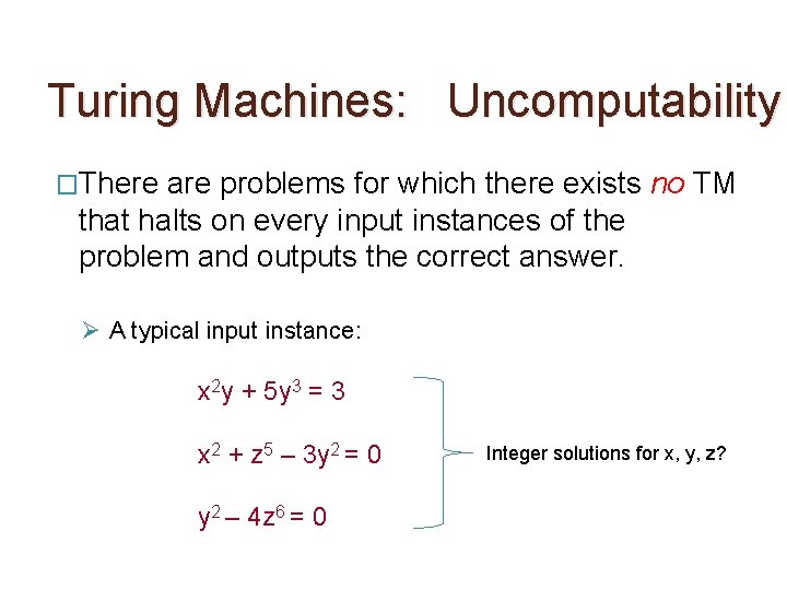
Turing Machines: Uncomputability �There are problems for which there exists no TM that halts on every input instances of the problem and outputs the correct answer. Ø A typical input instance: x 2 y + 5 y 3 = 3 x 2 + z 5 – 3 y 2 = 0 y 2 – 4 z 6 = 0 Integer solutions for x, y, z?

Turing Machines: Uncomputability �There are problems for which there exists no TM that halts on every input instances of the problem and outputs the correct answer. Ø Input: A system of polynomial equations in many variables with integer coefficients. Ø Output: Check if the system has integer solutions. Ø Question: Is there an algorithm to solve this problem? (Hilbert’s tenth problem, 1900)

Turing Machines: Uncomputability �There are problems for which there exists no TM that halts on every input instances of the problem and outputs the correct answer. Ø Input: A system of polynomial equations in many variables with integer coefficients. Ø Output: Check if the system has integer solutions. Ø Question: Is there an algorithm to solve this problem? � Theorem. There does not exist any algorithm (realizable by a TM) to solve this problem.

Why Turing Machines? �TMs are natural and intuitive. �Church-Turing thesis: “Every physically realizable computation device – whether it’s based on silicon, DNA, neurons or some other alien technology – can be simulated by a Turing machine”. --- [quoted from Arora-Barak’s book]

Why Turing Machines? �TMs are natural and intuitive. �Church-Turing thesis: “Every physically realizable computation device – whether it’s based on silicon, DNA, neurons or some other alien technology – can be simulated by a Turing machine”. --- [quoted from Arora-Barak’s book] �Several other computational models can be simulated by TMs.

Basic facts about TMs

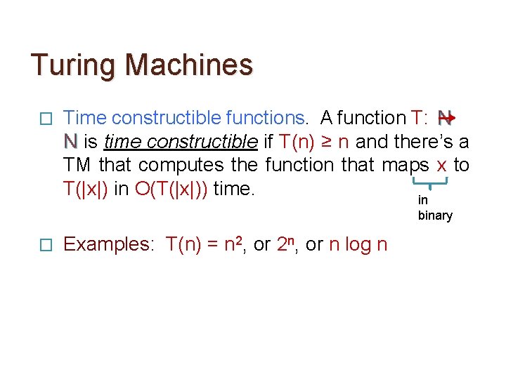
Turing Machines � Time constructible functions. A function T: N N is time constructible if T(n) ≥ n and there’s a TM that computes the function that maps x to T(|x|) in O(T(|x|)) time. in binary � Examples: T(n) = n 2, or 2 n, or n log n

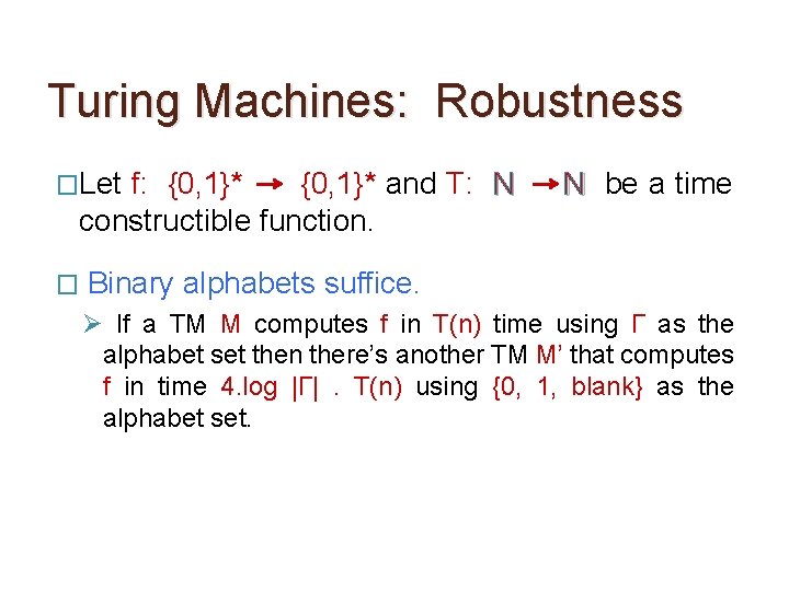
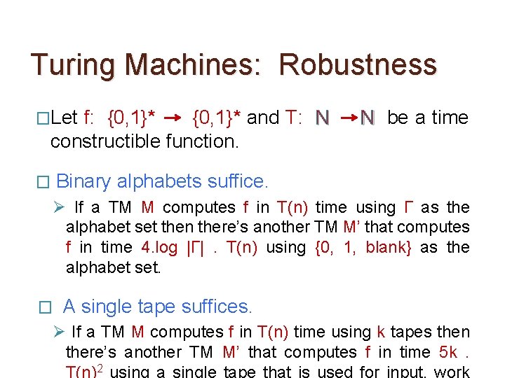
Turing Machines: Robustness �Let f: {0, 1}* and T: N constructible function. � N be a time Binary alphabets suffice. Ø If a TM M computes f in T(n) time using Γ as the alphabet set then there’s another TM M’ that computes f in time 4. log |Γ|. T(n) using {0, 1, blank} as the alphabet set.

Turing Machines: Robustness �Let f: {0, 1}* and T: N constructible function. N be a time Binary alphabets suffice. � Ø If a TM M computes f in T(n) time using Γ as the alphabet set then there’s another TM M’ that computes f in time 4. log |Γ|. T(n) using {0, 1, blank} as the alphabet set. � A single tape suffices. Ø If a TM M computes f in T(n) time using k tapes then there’s another TM M’ that computes f in time 5 k. T(n)2 using a single tape that is used for input, work

Turing Machines: As strings �Every TM can be represented by a finite string over {0, 1}. …simply encode the description of the TM.

Turing Machines: As strings �Every TM can be represented by a finite string over {0, 1}. �Every string over {0, 1} represents some TM. …invalid strings map to a fixed, trivial TM.

Turing Machines: As strings �Every TM can be represented by a finite string over {0, 1}. �Every string over {0, 1} represents some TM. �Every TM has infinitely many string representations. … allow padding with arbitrary number of 0’s

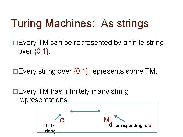
Turing Machines: As strings �Every TM can be represented by a finite string over {0, 1}. �Every string over {0, 1} represents some TM. �Every TM has infinitely many string representations. {0, 1} string α Mα TM corresponding to α

Turing Machines: As strings �Every TM can be represented by a finite string over {0, 1}. �Every string over {0, 1} represents some TM. �Every TM has infinitely many string representations. �A TM (i. e. its string representation) can be given as an input to another TM !!

Universal Turing Machines �Theorem. There exists a TM U that on every input x, α in {0, 1}* outputs Mα(x). �Further, if Mα halts within T steps then U halts within C. T. log T steps, where C is a constant that depends only on Mα ’s alphabet size, number of states and number of tapes.

Universal Turing Machines �Theorem. There exists a TM U that on every input x, α in {0, 1}* outputs Mα(x). �Further, if Mα halts within T steps then U halts within C. T. log T steps, where C is a constant that depends only on Mα ’s alphabet size, number of states and number of tapes. �Physical realization of UTMs are modern day electronic computers.