COMPUTATIONAL CHALLENGES WITH CLIQUES QUASICLIQUES AND CLIQUE PARTITIONS

COMPUTATIONAL CHALLENGES WITH CLIQUES, QUASICLIQUES AND CLIQUE PARTITIONS IN GRAPHS Panos M. Pardalos

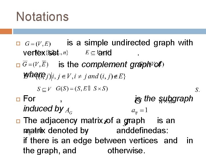
Notations is a simple undirected graph with vertex set and . is the complement graph of where For , is the subgraph induced by The adjacency matrix of a graph is an matrix denoted by and defined as: if there is an edge between vertices and in the graph, and otherwise.

Definitions A set of vertices S is called a clique if the subgraph G(S) induced by S is complete; i. e. there is an edge between any two vertices in G(S). A maximal clique is a clique which is not a proper subset of another clique. A maximum clique is a clique of the maximum cardinality.

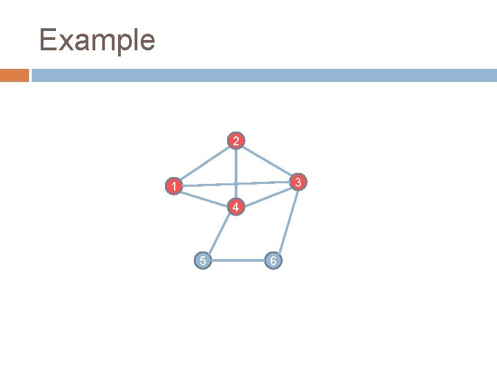
Example 2 3 1 4 5 6

The Maximum Clique Problem The maximum clique problem (MCP) is to find a maximum clique in a given graph G. We will denote the cardinality of the maximum clique in graph G by . The MCP is one of the classical problems in graph theory with many applications in many fields including project selection, classification, fault tolerance, coding, computer vision, economics, information retrieval, signal transmission, and alignment of DNA with protein sequences.

The Maximum Independent Set Problem A set of nodes S in a graph G is an independent set (stable set) if any two vertices in S are not adjacent. The maximum independent set problem is to find the independent set of the maximum cardinality. We denote the cardinality of this maximum independent set by .

The Minimum Vertex Cover Problem This is another optimization problem on graphs. A vertex cover is defined as a subset of the vertex set V such that every edge (i , j) in E has at least one endpoint in that subset. The minimum vertex cover problem asks for a vertex cover of minimum cardinality.

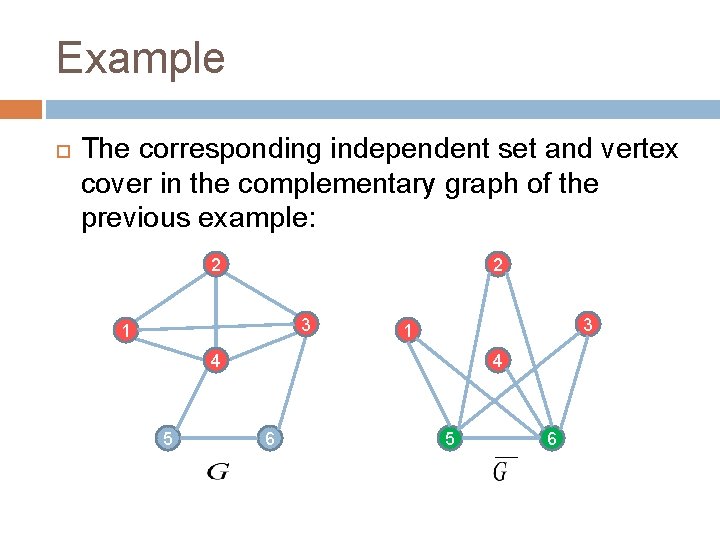
Equivalence An independent set in is a clique in and vice versa. Therefore, the two problems are equivalent. If S is an independent set in G, VS is a vertex cover of G. Therefore, the maximum independent set problem is equivalent to the minimum vertex cover problem. The above results show that these three problems are equivalent and therefore:

Example The corresponding independent set and vertex cover in the complementary graph of the previous example: 2 2 3 1 4 5 4 6 5 6

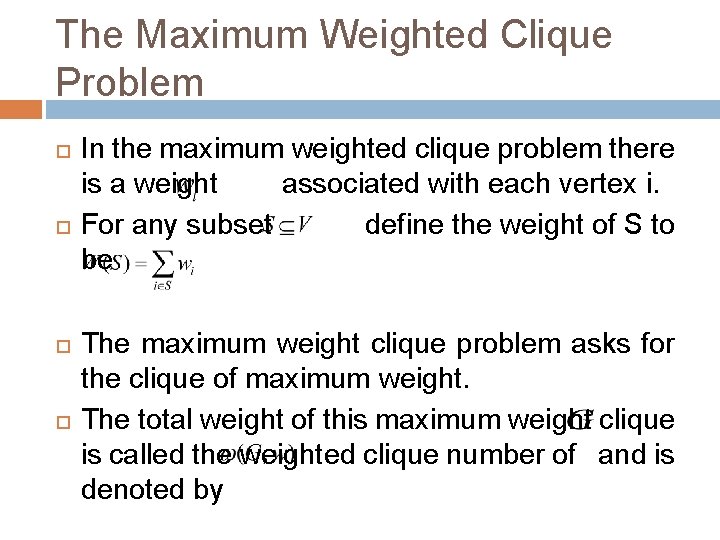
The Maximum Weighted Clique Problem In the maximum weighted clique problem there is a weight associated with each vertex i. For any subset define the weight of S to be The maximum weight clique problem asks for the clique of maximum weight. The total weight of this maximum weight clique is called the weighted clique number of and is denoted by

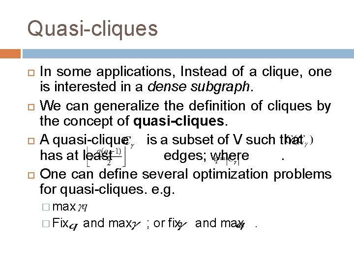
Quasi-cliques In some applications, Instead of a clique, one is interested in a dense subgraph. We can generalize the definition of cliques by the concept of quasi-cliques. A quasi-clique is a subset of V such that has at least edges; where . One can define several optimization problems for quasi-cliques. e. g. � max � Fix and max ; or fix and max .

Clique Relaxations According to Word. Net dictionary, clique is defined as “an exclusive circle of people with a common purpose”. Cliques, as described in the dictionary definition, represent a natural object of interest for social and behavioral sciences. It is not surprising that the first mentioning of this term in graph-theoretic context is attributed to researchers in social network analysis: in their 1949 paper, Luce and Perry used complete subgraphs to model cohesive subgroups

Clique Relaxations Desirable properties of cohesive subgroups: Familiarity (high degree of a vertex in the set) Reachability (small distance/diameter) Robustness (high connectivity) Clique model is ideal with respect to all these properties, however, it is overly restrictive

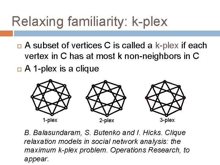
Relaxing familiarity: k-plex A subset of vertices C is called a k-plex if each vertex in C has at most k non-neighbors in C A 1 -plex is a clique 1 -plex 2 -plex 3 -plex B. Balasundaram, S. Butenko and I. Hicks. Clique relaxation models in social network analysis: the maximum k-plex problem. Operations Research, to appear.

Relaxing reachability A k-clique is a subset of vertices C such that the pairwise distance in G between any two vertices from C is at most k A k-club is a subset of vertices D that indices a subgraph of diameter at most k 1 -clique and 1 -club correspond to clique A k-club is always a k-clique, but the opposite may not be true

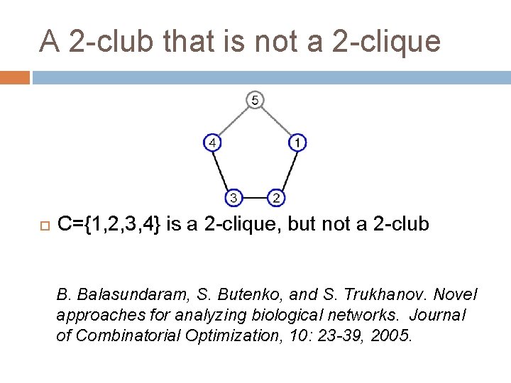
A 2 -club that is not a 2 -clique C={1, 2, 3, 4} is a 2 -clique, but not a 2 -club B. Balasundaram, S. Butenko, and S. Trukhanov. Novel approaches for analyzing biological networks. Journal of Combinatorial Optimization, 10: 23 -39, 2005.

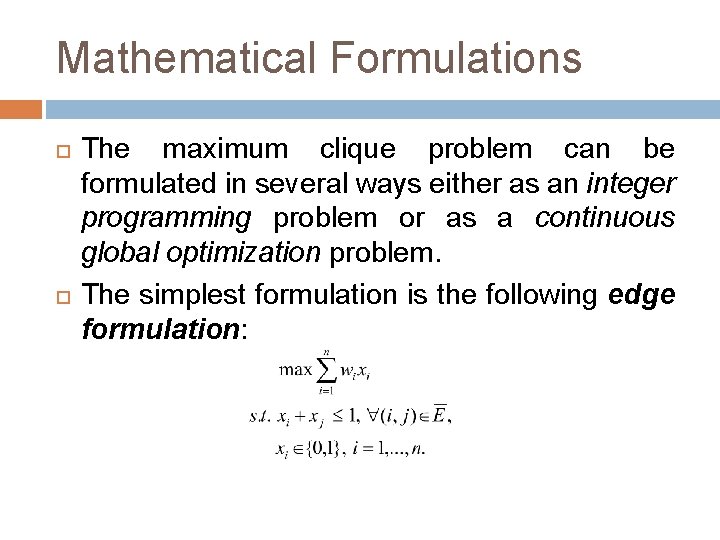
Mathematical Formulations The maximum clique problem can be formulated in several ways either as an integer programming problem or as a continuous global optimization problem. The simplest formulation is the following edge formulation:

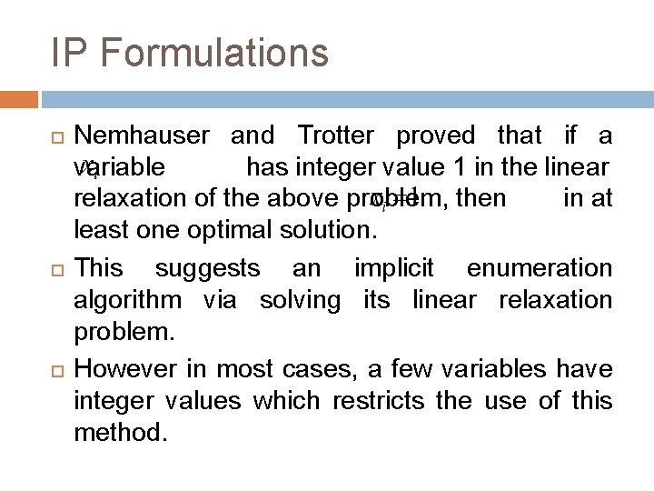
IP Formulations Nemhauser and Trotter proved that if a variable has integer value 1 in the linear relaxation of the above problem, then in at least one optimal solution. This suggests an implicit enumeration algorithm via solving its linear relaxation problem. However in most cases, a few variables have integer values which restricts the use of this method.

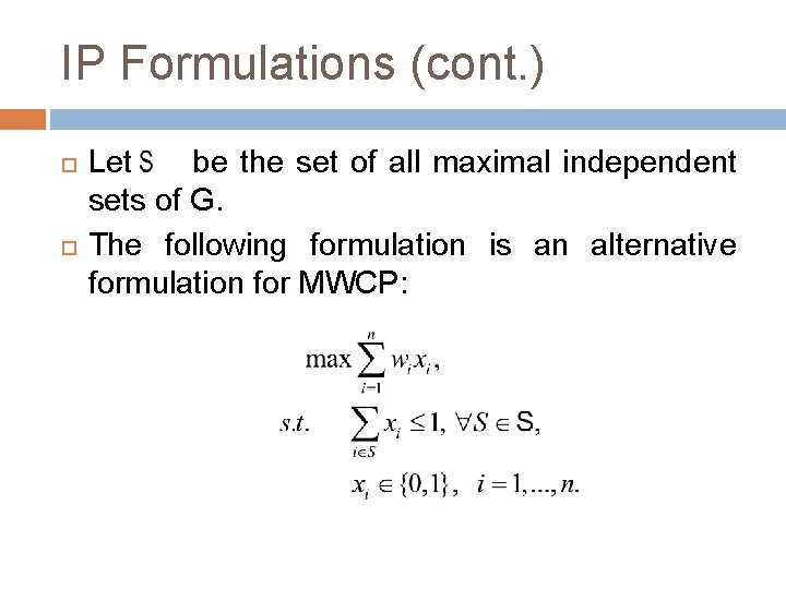
IP Formulations (cont. ) Let be the set of all maximal independent sets of G. The following formulation is an alternative formulation for MWCP:

IP Formulations (cont. ) The advantage of this formulation over the edge formulation is that it has a smaller relaxation gap. However, the exponential number constraints makes it a hard problem. of It has been proved that even the linear relaxation of this problem is NP-hard on general graphs.

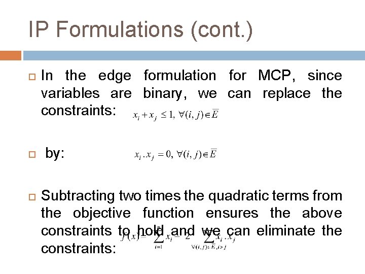
IP Formulations (cont. ) In the edge formulation for MCP, since variables are binary, we can replace the constraints: by: Subtracting two times the quadratic terms from the objective function ensures the above constraints to hold and we can eliminate the constraints:

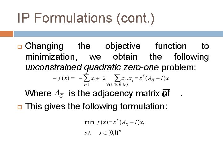
IP Formulations (cont. ) Changing the objective function to minimization, we obtain the following unconstrained quadratic zero-one problem: Where is the adjacency matrix of . This gives the following formulation:

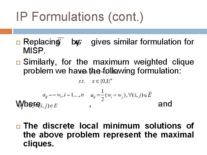
IP Formulations (cont. ) Replacing by gives similar formulation for MISP. Similarly, for the maximum weighted clique problem we have the following formulation: Where , and The discrete local minimum solutions of the above problem represent the maximal cliques.

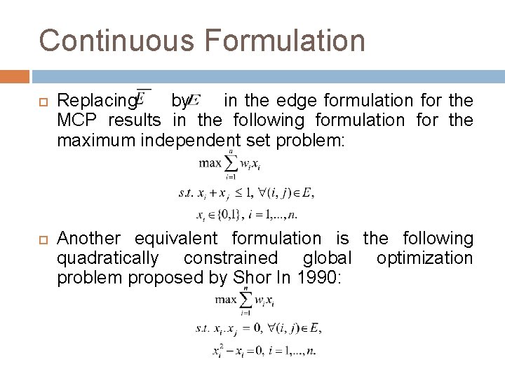
Continuous Formulation Replacing by in the edge formulation for the MCP results in the following formulation for the maximum independent set problem: Another equivalent formulation is the following quadratically constrained global optimization problem proposed by Shor In 1990:

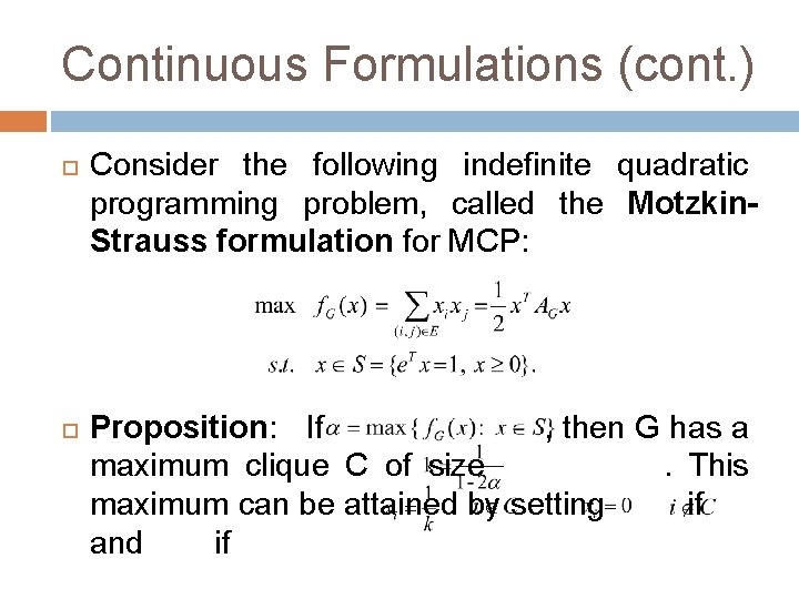
Continuous Formulations (cont. ) Consider the following indefinite quadratic programming problem, called the Motzkin. Strauss formulation for MCP: Proposition: If , then G has a maximum clique C of size . This maximum can be attained by setting if and if

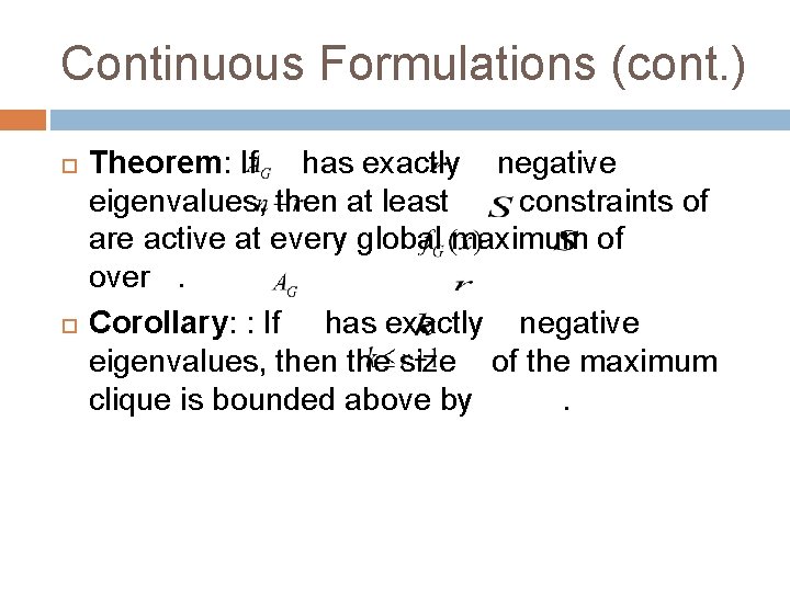
Continuous Formulations (cont. ) Theorem: If has exactly negative eigenvalues, then at least constraints of are active at every global maximum of over . Corollary: : If has exactly negative eigenvalues, then the size of the maximum clique is bounded above by .

Some References � P. M. Pardalos and A. T. Phillips. A global optimization approach for solving the maximum clique problem. International Journal of Computer Mathematics, Vol. 33 : 209 - 216, 1990. � R. Carraghan and P. M. Pardalos. An exact algorithm for the maximum clique problem. Operations Research Letters, Vol. 9 : 375 -382, 1990 (This algorithm was used in 1993 DIMACS implementation challenge). � P. M. Pardalos and G. P. Rodgers. A branch and bound algorithm for the maximum clique problem. Computers and Operations Research, Vol. 19: 363 -375, 1992.

Some References (cont. ) � S. Rebennack, M. Oswald, D. Theis, H. Seitz, G. Reinelt, P. M. Pardalos. A Branch and Cut solver for the maximum stable set problem. Journal of Combinatorial Optimization, to appear DOI: 10. 1007/s 10878 -009 -9264 -3. R.

Computational Complexity The MCP is one of the first problems shown to be NP-complete; i. e. unless P=NP, exact algorithms are guaranteed to return a solution only in a time which increases exponentially with the number of vertices in the graph. Arora and Safra proved that for some positive the approximation of the maximum clique within a factor of is NP-hard. The above fact along with practical evidence suggest that the maximum clique is hard to solve even in graphs of moderate sizes.

Enumerative Algorithms The first algorithm for enumerating all cliques of an arbitrary graph is due to Harray and Ross. In 1957, they proposed an inductive method that first identified all the cliques of a special graph with no more than three cliques. The problem on general graphs is reduced to this special case.

Enumerative Algorithms (cont. ) There are several other algorithms for enumerating all cliques in a graph. Some of these methods are called vertex sequence methods, which produce the cliques of G from the cliques of G{v}. Other algorithms are based on backtracking method, for example the algorithm proposed by Bron and Kerbosch.

Branch and Bound Algorithms have been widely used for solving the MCP and MWCP. There are three key issues in a branch-andbound algorithm for the maximum clique problem: � Finding a good lower bound, i. e. a clique of large size. � Finding a good upper bound on the size of the maximum clique. � How to branch, i. e. break a problem into smaller subproblems.

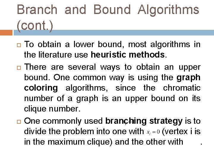
Branch and Bound Algorithms (cont. ) To obtain a lower bound, most algorithms in the literature use heuristic methods. There are several ways to obtain an upper bound. One common way is using the graph coloring algorithms, since the chromatic number of a graph is an upper bound on its clique number. One commonly used branching strategy is to divide the problem into one with (vertex i is in the maximum clique) and the other with .

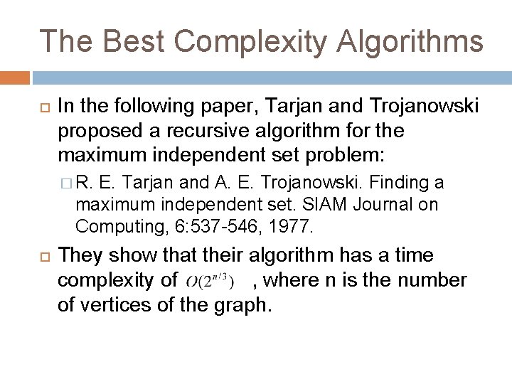
The Best Complexity Algorithms In the following paper, Tarjan and Trojanowski proposed a recursive algorithm for the maximum independent set problem: � R. E. Tarjan and A. E. Trojanowski. Finding a maximum independent set. SIAM Journal on Computing, 6: 537 -546, 1977. They show that their algorithm has a time complexity of , where n is the number of vertices of the graph.

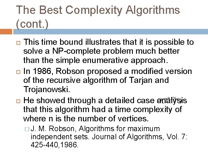
The Best Complexity Algorithms (cont. ) This time bound illustrates that it is possible to solve a NP-complete problem much better than the simple enumerative approach. In 1986, Robson proposed a modified version of the recursive algorithm of Tarjan and Trojanowski. He showed through a detailed case analysis that this algorithm had a time complexity of where n is the number of vertices. � J. M. Robson, Algorithms for maximum independent sets. Journal of Algorithms, Vol. 7: 425 -440, 1986.

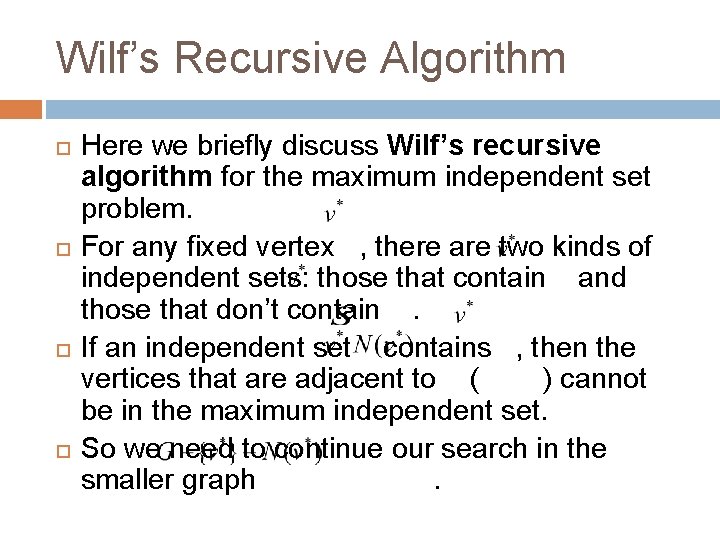
Wilf’s Recursive Algorithm Here we briefly discuss Wilf’s recursive algorithm for the maximum independent set problem. For any fixed vertex , there are two kinds of independent sets: those that contain and those that don’t contain . If an independent set contains , then the vertices that are adjacent to ( ) cannot be in the maximum independent set. So we need to continue our search in the smaller graph

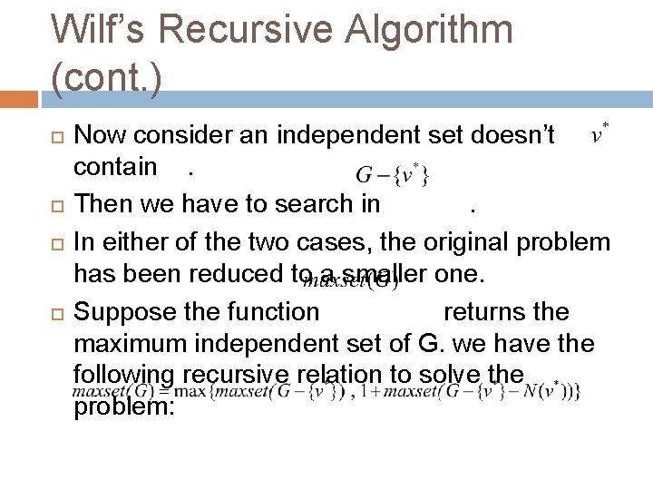
Wilf’s Recursive Algorithm (cont. ) Now consider an independent set doesn’t contain . Then we have to search in . In either of the two cases, the original problem has been reduced to a smaller one. Suppose the function returns the maximum independent set of G. we have the following recursive relation to solve the problem:

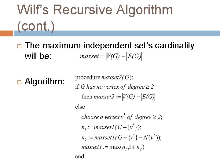
Wilf’s Recursive Algorithm (cont. ) We obtain the following recursive algorithm:

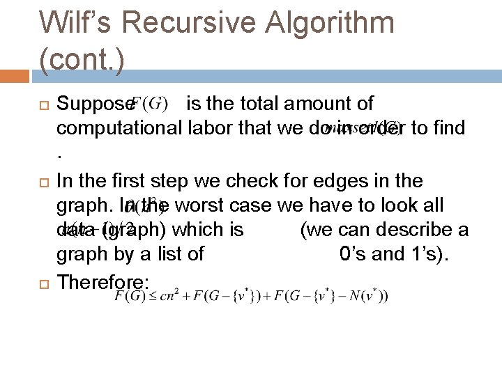
Wilf’s Recursive Algorithm (cont. ) Suppose is the total amount of computational labor that we do in order to find . In the first step we check for edges in the graph. In the worst case we have to look all data (graph) which is (we can describe a graph by a list of 0’s and 1’s). Therefore:

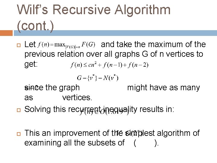
Wilf’s Recursive Algorithm (cont. ) Let and take the maximum of the previous relation over all graphs G of n vertices to get: since the graph might have as many as vertices. Solving this recurrent inequality results in: This an improvement of the simplest algorithm of examining all the subsets of ( ).

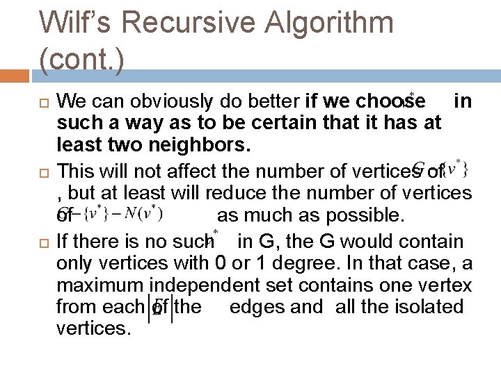
Wilf’s Recursive Algorithm (cont. ) We can obviously do better if we choose in such a way as to be certain that it has at least two neighbors. This will not affect the number of vertices of , but at least will reduce the number of vertices of as much as possible. If there is no such in G, the G would contain only vertices with 0 or 1 degree. In that case, a maximum independent set contains one vertex from each of the edges and all the isolated vertices.

Wilf’s Recursive Algorithm (cont. ) The maximum independent set’s cardinality will be: Algorithm:

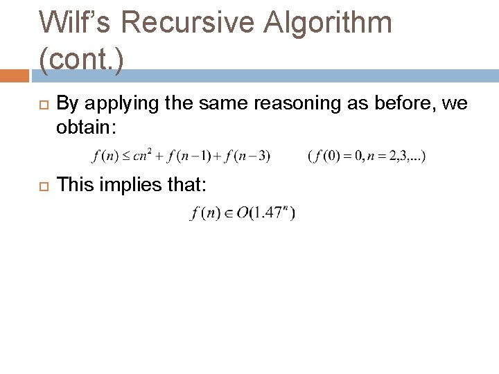
Wilf’s Recursive Algorithm (cont. ) By applying the same reasoning as before, we obtain: This implies that:

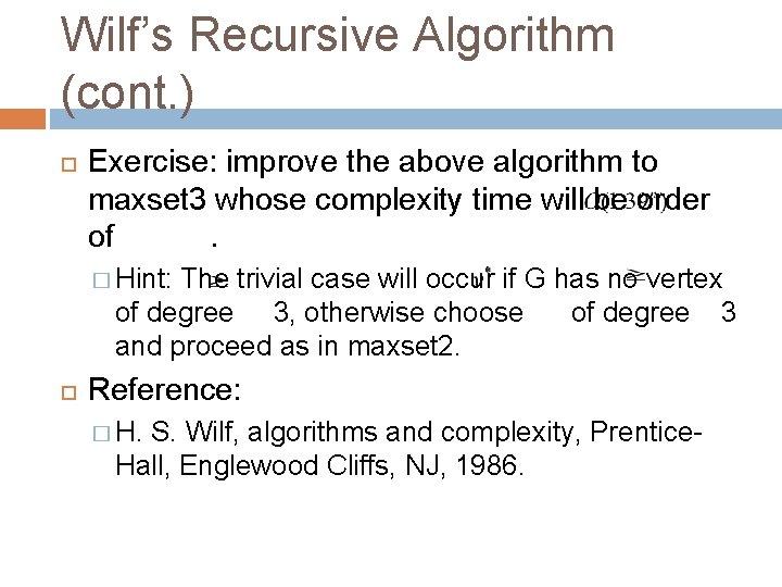
Wilf’s Recursive Algorithm (cont. ) Exercise: improve the above algorithm to maxset 3 whose complexity time will be order of . � Hint: The trivial case will occur if G has no vertex of degree 3, otherwise choose of degree 3 and proceed as in maxset 2. Reference: � H. S. Wilf, algorithms and complexity, Prentice- Hall, Englewood Cliffs, NJ, 1986.

Heuristics Because of the computational complexity of the maximum clique problem, much effort has been directed towards devising efficient heuristics. The main drawback of these heuristic is that usually there is no theoretical guarantee on their performance. Therefore, their evaluation is based essentially based on massive experimentation.

Heuristics (cont. ) There are several local search heuristics for the maximum clique problem. Although most of these heuristics find globally optimal solutions, the main difficulty is the fact that we cannot verify global optimality (lack of certificate of optimality). Therefore, many variations of the basic local search procedure has been devised which try to avoid local optima.

Heuristics (cont. ) Several examples of such metaheuristic methods that has been applied to the maximum clique problem: � Simulated Annealing � Neural Networks � Genetic Algorithms � Tabu Search

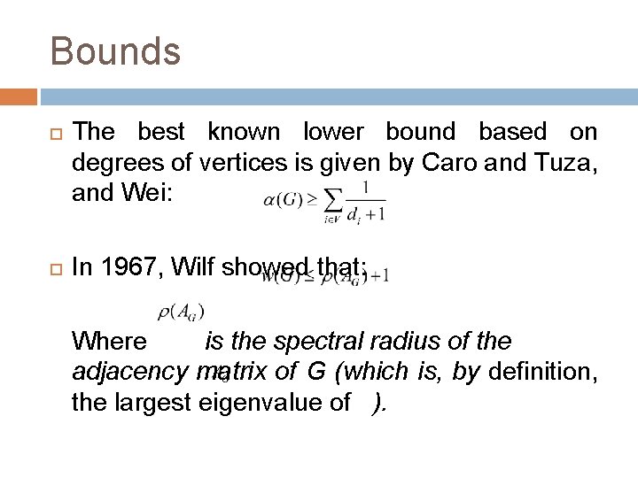
Bounds The best known lower bound based on degrees of vertices is given by Caro and Tuza, and Wei: In 1967, Wilf showed that: Where is the spectral radius of the adjacency matrix of G (which is, by definition, the largest eigenvalue of ).

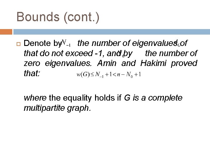
Bounds (cont. ) Denote by the number of eigenvalues of that do not exceed -1, and by the number of zero eigenvalues. Amin and Hakimi proved that: where the equality holds if G is a complete multipartite graph.

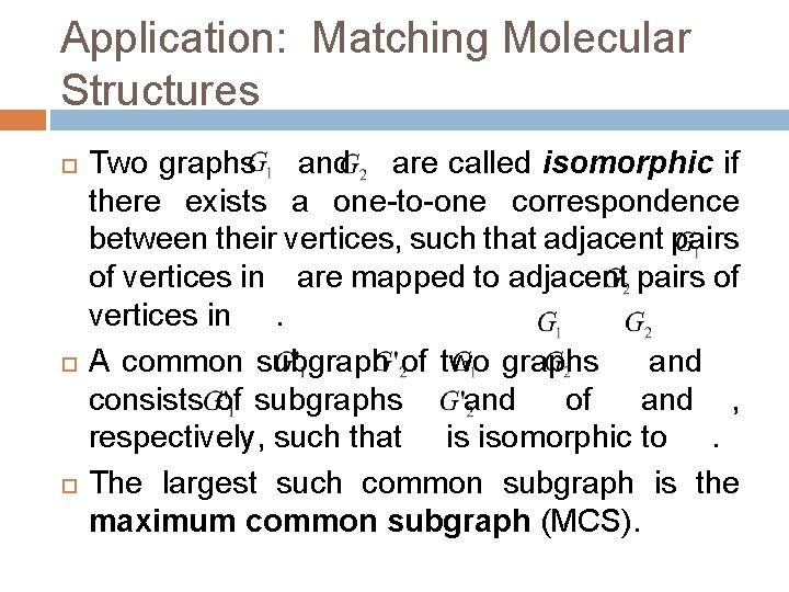
Application: Matching Molecular Structures Two graphs and are called isomorphic if there exists a one-to-one correspondence between their vertices, such that adjacent pairs of vertices in are mapped to adjacent pairs of vertices in . A common subgraph of two graphs and consists of subgraphs and of and , respectively, such that is isomorphic to . The largest such common subgraph is the maximum common subgraph (MCS).

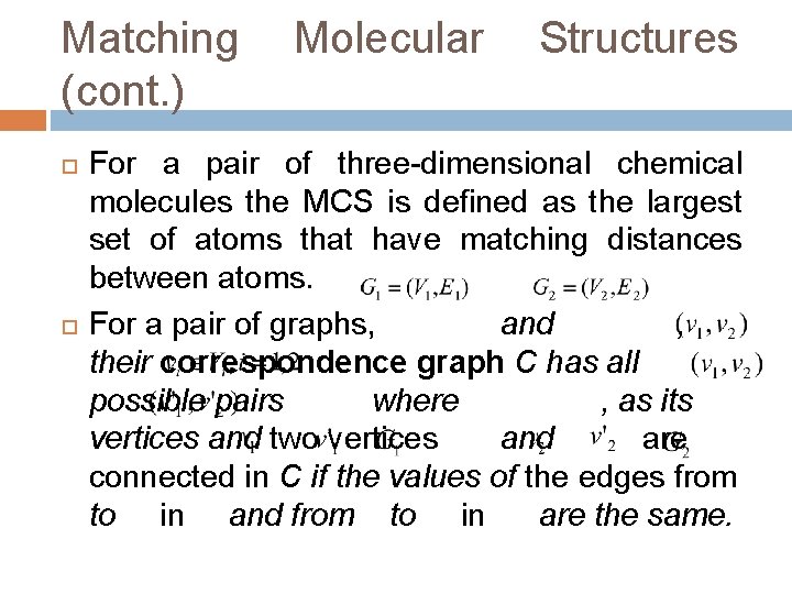
Matching Molecular Structures (cont. ) For a pair of three-dimensional chemical molecules the MCS is defined as the largest set of atoms that have matching distances between atoms. For a pair of graphs, and , their correspondence graph C has all possible pairs where , as its vertices and two vertices and are connected in C if the values of the edges from to in and from to in are the same.

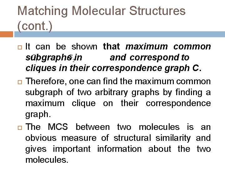
Matching Molecular Structures (cont. ) It can be shown that maximum common subgraphs in and correspond to cliques in their correspondence graph C. Therefore, one can find the maximum common subgraph of two arbitrary graphs by finding a maximum clique on their correspondence graph. The MCS between two molecules is an obvious measure of structural similarity and gives important information about the two molecules.

Challenging Problem Algorithm for Correspondence Graphs with Low Density Design an efficient algorithm for the maximum clique problem tailored to correspondence graphs resulting from matching of three-dimensional chemical molecules.

Matching Molecular Structures (cont. ) Details about this method can be found in: � E. Gardiner, P. Artymiuk, and P. Willett. Clique- detection algorithms for matching threedimensional molecular structures. Journal of Molecular Graphics and Modelling, 15: 245– 253, 1997.

Application: Docking Macromolecular Given two proteins, the protein docking problem is to find whether they interact to form a stable complex, and if they do, then how. This problem is fundamental to all aspects of biological function. Given two proteins, the docking problem can be experimentally solved.

Macromolecular Docking (cont. ) However, the large number of known protein structures urges the need for development of reliable theoretical protein docking techniques. One of the approaches to the macromolecular docking problem consists in representing each of two proteins as a set of potential hydrogen bond donors and acceptors and using a clique-detection algorithm to find maximally complementary sets of donor/acceptor pairs.

Macromolecular Docking (cont. ) Details about this topic can be found in: � E. Gardiner, P. Willett, and P. Artymiuk. Graph- theoretic techniques for macromolecular docking. J. Chem. Inf. Comput. , 40: 273– 279, 2000.

Comparative Modeling of Protein Structure The rapidly growing number of known protein structures requires the construction of accurate comparative models. Proteins are large organic compounds made of amino acids arranged in a linear chain and joined together. Each of these amino acids is called a residue. Each residue has several possible conformations. We can compare different protein structures using clique finding algorithms.

Comparative Modeling of Protein Structure (cont. ) We construct a graph in which vertices correspond to each possible conformation of a residue in an amino acid sequence. Edges connect pairs of residue conformations (vertices) that are consistent with each other; i. e. clash-free and satisfying geometrical constraints. Edges are drawn between different residue conformations; so that there is no edge between to different conformations of a single residue.

Comparative Modeling of Protein Structure (cont. ) Based on the strength of interaction between the atoms corresponding to the two vertices, weights are assigned to the edges. Then the cliques with the largest weights in the constructed graph represent the optimal combination of the various main-chain and side-chain possibilities, taking the respective environments into account.

Applications in Clustering The essence of clustering is partitioning the elements in a certain dataset into several distinct subsets (clusters) grouped according to an appropriate similarity criterion The retrieval of similar data is an obvious application of the maximum clique problem. A graph is constructed with vertices corresponding to data items and the edges connect vertices that are similar. A clique in such a graph is a cluster.

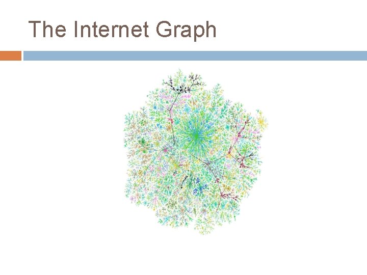
MCP in Very Large Graphs The graphs we have to deal with in some applications are very massive. Examples are the WWW graph and a call graph. The various gigantic graphs that have lately attracted notice share some properties: � They tend to be sparse: The graphs have relatively few edges, considering their vast numbers of vertices. � They tend to be clustered. In the World Wide Web, two pages that are linked to the same page have an elevated probability of including links to one another.

MCP in Very Large Graphs (cont. ) � They tend to have a small diameter. The diameter of a graph is the longest shortest path across it. Graphs nearer to the minimum than the maximum number of edges might be expected to have a large diameter. Nevertheless, the diameter of the Web and other big graphs seems to hover around the logarithm of n, which is much smaller than n itself. Graphs with the three properties of sparseness, clustering and small diameter have been termed "small-world" graphs.

The Internet Graph

MCP in Very Large Graphs (cont. ) In many cases, the data associated with massive graphs is too large to fit entirely inside the computer’s internal memory. Therefore a slower external memory (for example disks) needs to be used. The input/output communication (I/O) between these memories can result in an algorithm’s slow performance.

The Call Graph In the call graph, the vertices are telephone numbers, and two vertices are connected by an edge if a call was made from one number to another. A call graph was constructed with data from AT&T telephone billing records. Based on one 20 -day period it had 290 million vertices and 4 billion edges. The analyzed one-day call graph had 53, 767, 087 vertices and over 170 millions of edges

The Call Graph (cont. ) This graph appeared to have 3, 667, 448 connected components, most of them tiny. A giant connected component with 44, 989, 297 vertices (more than 80 percent of the total) was computed. The distribution of the degrees of the vertices follows the power-law distribution (see later discussion).

A GRASP-Based Algorithm In the call graph, the only feasible strategy to find the cliques is a probabilistic search that finds large cliques without proving them maximal. GRASP is an iterative method that at each iteration constructs, using a greedy function, a randomized solution and then finds a locally optimal solution by searching the neighborhood of the constructed solution. This is a heuristic approach which gives no guarantee about quality of the solutions found, but proved to be practically efficient for many combinatorial optimization problems.

A GRASP-Based Algorithm (cont. ) To describe a GRASP, one needs to specify a construction mechanism and a local search procedure. The construction phase of the GRASP for maximum clique problem builds a clique, one vertex at a time. It uses vertex degrees as a guide for construction and constructs a clique in a greedy manner.

A GRASP-Based Algorithm (cont. ) In each step, the algorithm selects the vertex with the highest degree, and then updates the graph by eliminating all the vertices which are not connected to the selected vertex. Local search can be implemented in many ways. A simple (2, 1) -exchange approach seeks a vertex in the clique whose removal allows two adjacent vertices not in the clique to be included in the clique, thus increasing the clique size by one.

A GRASP-Based Algorithm (cont. ) Using this local search approach, we can search the feasible region and find local optimal solutions. Repeating this procedure several times, we can find a clique of large size. The GRASP described in this section requires access to the edges and vertices of the graph. This limits use to graphs small enough to fit in memory.

A GRASP-Based Algorithm (cont. ) We can develop a semi-external procedure that works only with vertex degrees and a subset of the edges in-memory, while most of the edges can be kept in secondary disk storage. The procedure starts with applying GRASP to the graph induced by a subset of edges. This gives us a clique with size q. Because vertices with degree less than q cannot be in a maximum clique, we can eliminate those and apply the algorithm to the reduced graph.

A GRASP-Based Algorithm (cont. ) The algorithm continues to run these two steps until no more reduction is possible. Reducing the size of the graph allows GRASP to explore portions of the solution space at greater depth, since GRASP iterations are faster on smaller graphs. Using the above algorithm, Abello et al. found cliques of size 30 in the call graph, which are almost surely the largest. Remarkably, there are more than 14, 000 of these 30 -member cliques.

MCP in Very Large Graphs (cont. ) The size of real-life massive graphs, many of which cannot be held even by a computer with several gigabytes of main memory, vanishes the power of classical algorithms and makes one look for novel approaches. In some cases not only is the amount of data huge, but the data itself is not completely available. e. g. the largest search engines are estimated to cover only 38% of the Web.

MCP in Very Large Graphs (cont. ) Some approaches were developed for studying the properties of real-life massive graphs using only the information about a small part of the graph. Another methodology of investigating real-life massive graphs is to use the available information in order to construct proper theoretical models of these graphs. One of the earliest attempts to model real networks theoretically goes back to the late 1950’s, when the foundations of random graph theory had been developed.

Random Graphs One way to model massive datasets is uniform random graphs. One example of uniform graphs is as follows: each pair of vertices is chosen to be linked by an edge randomly and independently with probability p. There also more general ways of modeling random graphs which deal with random graphs with a given degree sequence. One important model of such random graphs with a given degree sequence is the power-law random graph model.

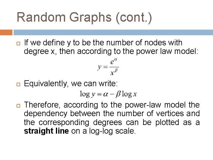
Random Graphs (cont. ) If we define y to be the number of nodes with degree x, then according to the power law model: Equivalently, we can write: Therefore, according to the power-law model the dependency between the number of vertices and the corresponding degrees can be plotted as a straight line on a log-log scale.

The Call Graph (cont. ) Aiello, Chung and Lu investigated the same call graph that was analyzed by Abello et al. Comparison between the experimental results presented by Abello et al. with theoretical results obtained by Aiello et al. shows that the power-law model fairly well describes some of the real-life massive graphs, such as the call graph.

Challenging Problem Algorithm for Massive Graphs with Very Low Density Design an efficient algorithm together with a data base for the maximum –clique problem tailored to massive graphs characterized by very low density and by the node degree distribution following a power-law. Real world call graphs serve as an excellent test bed.

The Call Graph (cont. ) Some references for further study: � J. Abello, P. M. Pardalos, and M. G. C. Resende. On maximum clique problems in very large graphs. In J. Abello and J. S. Vitter, editors. External Memory Algorithms, pages 119– 130. � J Abello, PM Pardalos, MGC Resende. Handbook of massive data sets. Dordrecht, The Netherlands: Kluwer, 2002.

The Call Graph (cont. ) American Scientist (January-February 2000, Volume 88, No. 1), “Computing Science Graph Theory in Practice: Part I by Brian Hayes” (http: //www. americanscientist. org/issues/pub/graphtheory-in-practice-part-ii/1) American Scientist (September-October 2006, Volume 94, Number 5), “Connecting the Dots: Can the tools of graph theory and social-network studies unravel the next big plot? ” (http: //www. americanscientist. org/issues/pub/connect ing-the-dots/1)

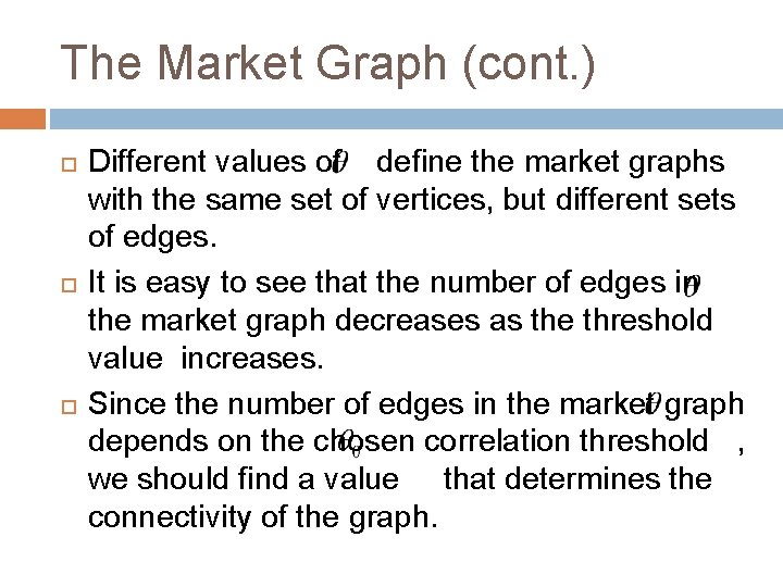
The Market Graph Financial markets can also be represented as graphs. For a stock market one natural representation is based on the cross correlations of stock price fluctuations. Each stock is represented by a vertex, and two vertices are connected by an edge if the correlation coefficient of the corresponding pair of stocks (calculated for a certain period of time) is above a prespecified threshold .

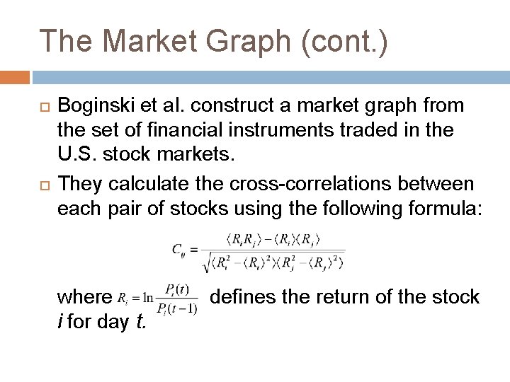
The Market Graph (cont. ) Boginski et al. construct a market graph from the set of financial instruments traded in the U. S. stock markets. They calculate the cross-correlations between each pair of stocks using the following formula: where defines the return of the stock i for day t.

The Market Graph (cont. ) Different values of define the market graphs with the same set of vertices, but different sets of edges. It is easy to see that the number of edges in the market graph decreases as the threshold value increases. Since the number of edges in the market graph depends on the chosen correlation threshold , we should find a value that determines the connectivity of the graph.

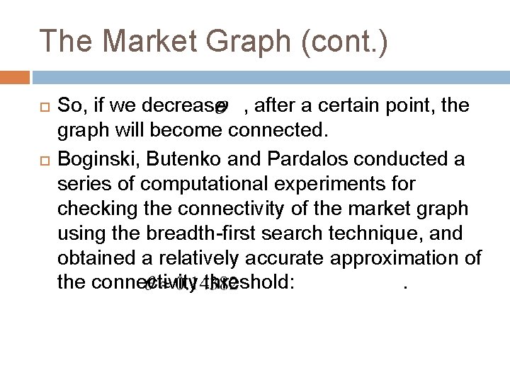
The Market Graph (cont. ) So, if we decrease , after a certain point, the graph will become connected. Boginski, Butenko and Pardalos conducted a series of computational experiments for checking the connectivity of the market graph using the breadth-first search technique, and obtained a relatively accurate approximation of the connectivity threshold: .

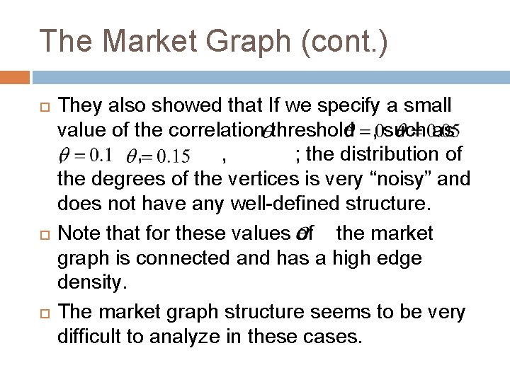
The Market Graph (cont. ) They also showed that If we specify a small value of the correlation threshold , such as , , ; the distribution of the degrees of the vertices is very “noisy” and does not have any well-defined structure. Note that for these values of the market graph is connected and has a high edge density. The market graph structure seems to be very difficult to analyze in these cases.

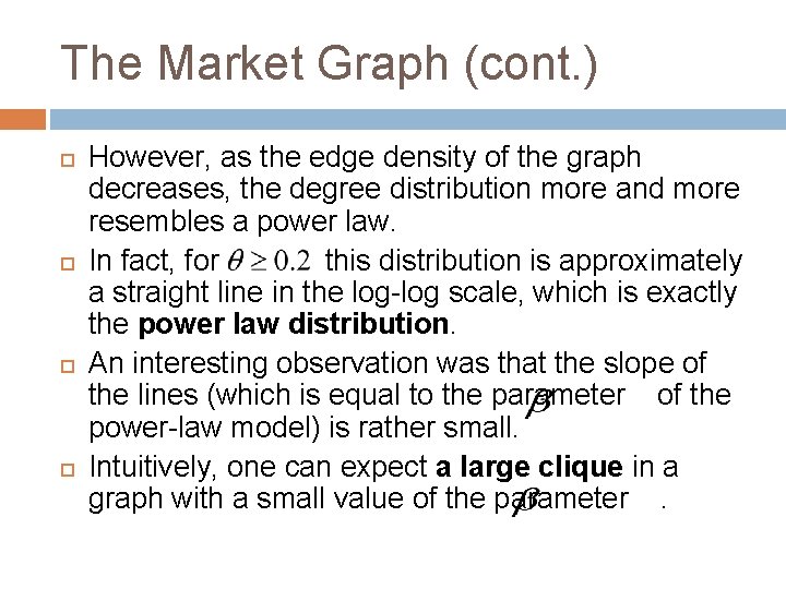
The Market Graph (cont. ) However, as the edge density of the graph decreases, the degree distribution more and more resembles a power law. In fact, for this distribution is approximately a straight line in the log-log scale, which is exactly the power law distribution. An interesting observation was that the slope of the lines (which is equal to the parameter of the power-law model) is rather small. Intuitively, one can expect a large clique in a graph with a small value of the parameter .

The Market Graph (cont. ) Another combinatorial optimization problem associated with the market graph is finding maximum independent sets in the graphs with a negative correlation threshold . Clearly, instruments in an independent set will be negatively correlated with each other, and therefore form a diversified portfolio. The financial interpretation of the clique in the market graph is that it defines the set of stocks whose price fluctuations exhibit a similar behavior.

The Market Graph (cont. ) In the modern stock market there are large groups of instruments that are correlated with each other. References: � Boginski V, Butenko S, Pardalos PM. On structural properties of the market graph. In: Nagurney A, editor. Innovations in financial and economic networks. Edward Elgar Publishers; 2003. � Boginski V, Butenko S, Pardalos PM. Statistical analysis of financial networks. Computational Statistics and Data Analysis 2005; 48(2): 431– 43. � Boginski V, Butenko S, Pardalos PM. Mining market data: A network approach. Computers & Operations Research, 33: 3171 -3184, 2006.

Recent results A. Vizgunov, B. Goldengorin, V. Kalyagin, A. Koldanov, P. M. Pardalos. Network approach for the Russian stock market. Computational Management Science, DOI 10. 1007/s 10287 -013 -0165 -7, 2013. Abstract We consider a market graph model of the Russian stock market. To study the peculiarity of the Russian market we construct the market graphs for different time periods from 2007 to 2011. As characteristics of constructed market graphs we use the distribution of correlations, size and structure of maximum cliques, and relationship between return and volume of stocks. Our main finding is that for the Russian market there is a strong connection between the volume of stocks and the structure of maximum cliques for all periods of observations. Namely, the most attractive Russian stocks have a strongest correlation between their returns. At the same time as far as we are aware this phenomenon is not related to the well developed USA stock market.

Recent results Grigory A. Bautin, Valery A. Kalyagin, Alexander P. Koldanov, Petr A. Koldanov, Panos M. Pardalos. Simple measure of similarity for the market graph construction. Computational Management Science, DOI 10. 1007/s 10287 -013 -0169 -3, 2013. Abstract A simple measure of similarity for the construction of the market graph is proposed. The measure is based on the probability of the coincidence of the signs of the stock returns. This measure is robust, has a simple interpretation, is easy to calculate and can be used as measure of similarity between any number of random variables. For the case of pairwise similarity the connection of this measure with the sign correlation of Fechner is noted. The properties of the proposed measure of pairwise similarity in comparison with the classic Pearson correlation are studied. The simple measure of pairwise similarity is applied (in parallel with the classic correlation) for the study of Russian and Swedish market graphs. The new measure of similarity for more than two random variables is introduced and applied to the additional deeper analysis of Russian and Swedish markets. Some interesting phenomena for the cliques and independent sets of the obtained market graphs are observed.

Vertex Coloring Problem A proper (vertex) coloring of G is an assignment of colors to its vertices so that no pair of adjacent vertices has the same color. If there exists a coloring of G that uses no more than k colors, we say that G admits a kcoloring. The minimal k for which G admits a k-coloring is called the chromatic number and is denoted by . The graph coloring problem is to find as well as the partition of vertices induced by a

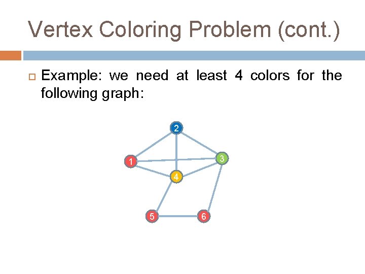
Vertex Coloring Problem (cont. ) Example: we need at least 4 colors for the following graph: 2 3 1 4 5 6

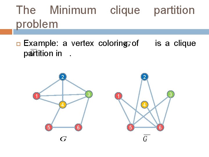
The Minimum clique partition problem is to partition vertices of a graph G into minimum number of cliques. In fact, a coloring induces a partition of the vertex set such that the elements of each set in the partition are pairwise nonadjacent. In the complement graph , this means a partition of vertex set into cliques. Therefore, minimum clique partition problem and vertex coloring problem are equivalent.

The Minimum clique partition problem Example: a vertex coloring of is a clique partition in . 2 2 3 1 4 5 4 6 5 6

Example: Covering Locations Given a set of demand points and a set of potential sites for locating facilities, a demand point is said to be covered by a facility if it is located within a pre-specified distance from that facility. Mandatory coverage problems aim to cover all demand points with the minimum number of facilities. Here, we consider an application of mandatory coverage problem arising in cytological screening tests for cervical cancer.

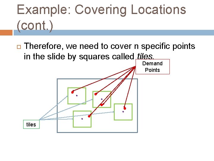
Example: Covering Locations (cont. ) In this application, a cervical specimen on a glass slide has to be viewed by a screener device. The screener is relocated on the glass slide in order to explore n demand points in the specimen. The goal is to minimize the number of viewing locations (sites). The area covered by the screener is a square and screener can move in any of four directions parallel to the sides of the

Example: Covering Locations (cont. ) Therefore, we need to cover n specific points in the slide by squares called tiles. Demand Points tiles

Example: Covering Locations (cont. ) 1. 2. Interestingly, this problem can be formulated as minimum clique partition problem. Lemma: The following two statements are equivalent: There exists a covering of n demand points in the rectangle using k tiles. Given n tiles centered in the demand points, there exist k points in the rectangle such that each of the tiles contains at least one of them.

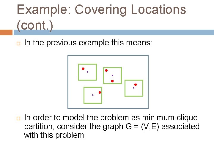
Example: Covering Locations (cont. ) In the previous example this means: In order to model the problem as minimum clique partition, consider the graph G = (V, E) associated with this problem.

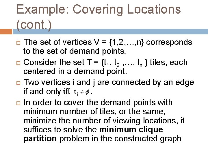
Example: Covering Locations (cont. ) The set of vertices V = {1, 2, …, n} corresponds to the set of demand points. Consider the set T = {t 1, t 2 , …, tn } tiles, each centered in a demand point. Two vertices i and j are connected by an edge if and only if . In order to cover the demand points with minimum number of tiles, or the same, minimize the number of viewing locations, it suffices to solve the minimum clique partition problem in the constructed graph

Example: Covering Locations (cont. ) Details about this example can be found in the following: � L. Brotcorne, G. Laporte, and F. Semet. Fast heuristic for large scale covering location problems. Computers & Operations Research, 29: 651– 665, 2002.

Applications in Coding Theory Error correcting codes lie in the heart of digital technology; making cell phones, compact disk players and modems possible. A fundamental problem of interest is to send a message across a noisy channel with a maximum possible reliability. In coding theory, one wishes to find a binary code as large as possible that can correct a certain number of errors for a given size of the binary words (vectors).

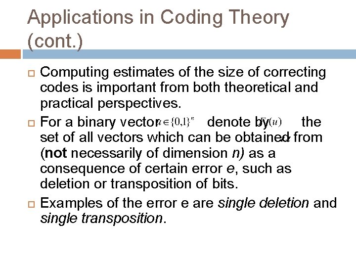
Applications in Coding Theory (cont. ) Computing estimates of the size of correcting codes is important from both theoretical and practical perspectives. For a binary vector denote by the set of all vectors which can be obtained from (not necessarily of dimension n) as a consequence of certain error e, such as deletion or transposition of bits. Examples of the error e are single deletion and single transposition.

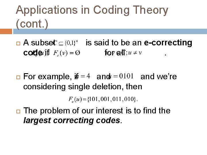
Applications in Coding Theory (cont. ) A subset is said to be an e-correcting code if for all . For example, if and we’re considering single deletion, then The problem of our interest is to find the largest correcting codes.

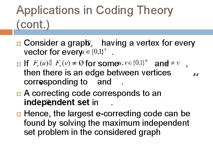
Applications in Coding Theory (cont. ) Consider a graph having a vertex for every vector for every . If for some and , then there is an edge between vertices corresponding to and . A correcting code corresponds to an independent set in . Hence, the largest e-correcting code can be found by solving the maximum independent set problem in the considered graph

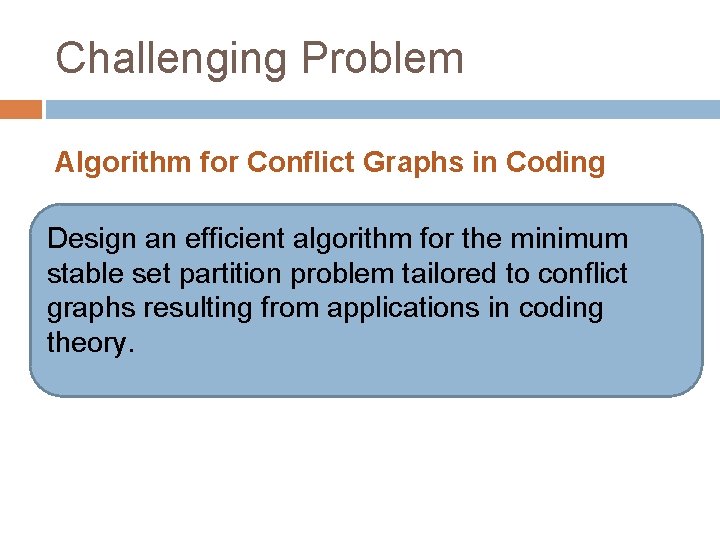
Challenging Problem Algorithm for Conflict Graphs in Coding Theory Design an efficient algorithm for the minimum stable set partition problem tailored to conflict graphs resulting from applications in coding theory.

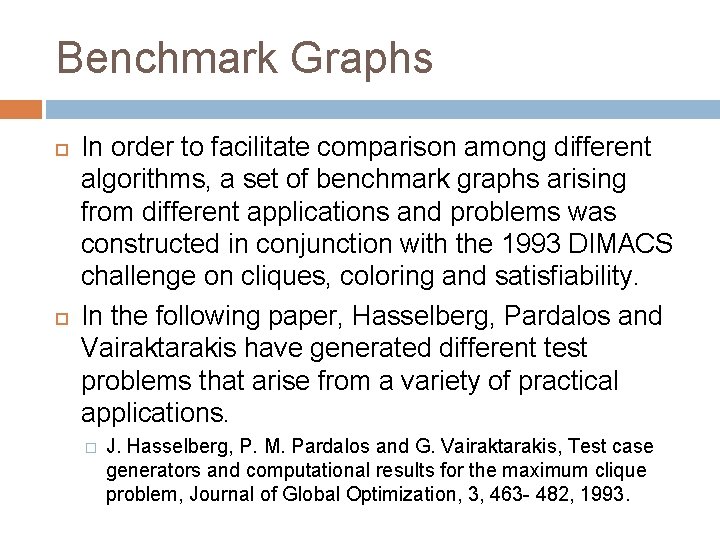
Benchmark Graphs In order to facilitate comparison among different algorithms, a set of benchmark graphs arising from different applications and problems was constructed in conjunction with the 1993 DIMACS challenge on cliques, coloring and satisfiability. In the following paper, Hasselberg, Pardalos and Vairaktarakis have generated different test problems that arise from a variety of practical applications. � J. Hasselberg, P. M. Pardalos and G. Vairaktarakis, Test case generators and computational results for the maximum clique problem, Journal of Global Optimization, 3, 463 - 482, 1993.

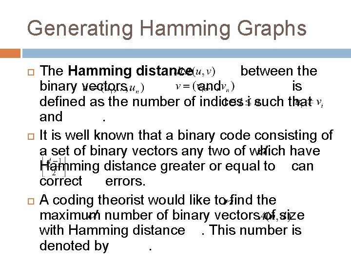
Generating Hamming Graphs The Hamming distance between the binary vectors and is defined as the number of indices i such that and . It is well known that a binary code consisting of a set of binary vectors any two of which have Hamming distance greater or equal to can correct errors. A coding theorist would like to find the maximum number of binary vectors of size with Hamming distance . This number is denoted by .

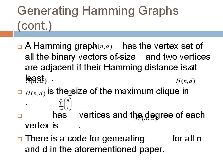
Generating Hamming Graphs (cont. ) A Hamming graph has the vertex set of all the binary vectors of size and two vertices are adjacent if their Hamming distance is at least . is the size of the maximum clique in . has vertices and the degree of each vertex is . There is a code for generating for all n and d in the aforementioned paper.

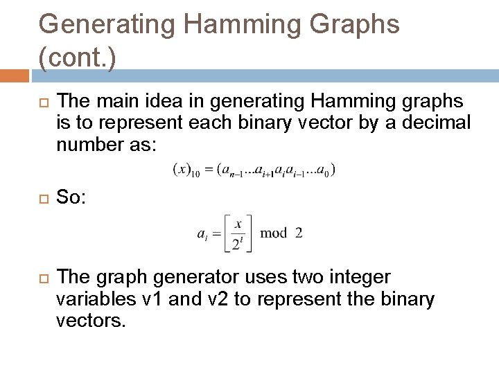
Generating Hamming Graphs (cont. ) The main idea in generating Hamming graphs is to represent each binary vector by a decimal number as: So: The graph generator uses two integer variables v 1 and v 2 to represent the binary vectors.

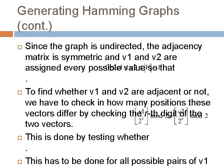
Generating Hamming Graphs (cont. ) Since the graph is undirected, the adjacency matrix is symmetric and v 1 and v 2 are assigned every possible value so that . To find whether v 1 and v 2 are adjacent or not, we have to check in how many positions these vectors differ by checking the r-th digit of the two vectors. This is done by testing whether . This has to be done for all possible pairs of v 1

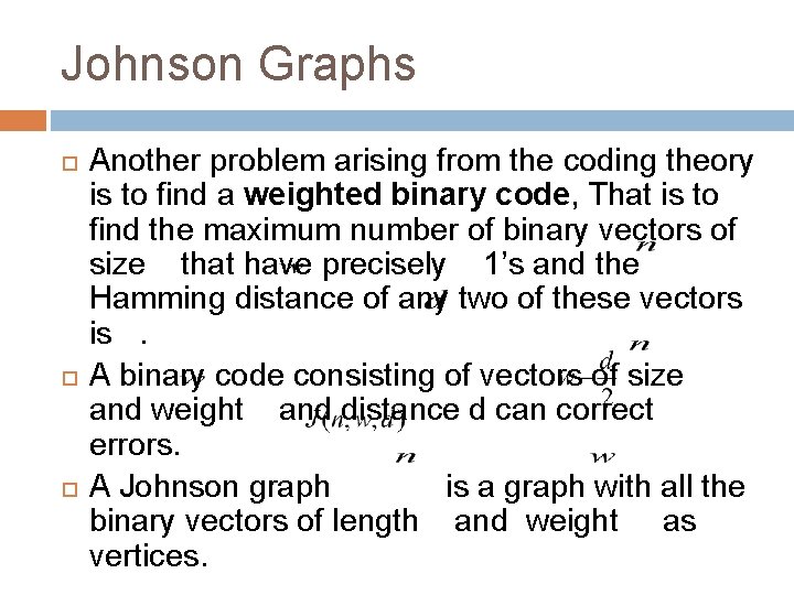
Johnson Graphs Another problem arising from the coding theory is to find a weighted binary code, That is to find the maximum number of binary vectors of size that have precisely 1’s and the Hamming distance of any two of these vectors is . A binary code consisting of vectors of size and weight and distance d can correct errors. A Johnson graph is a graph with all the binary vectors of length and weight as vertices.

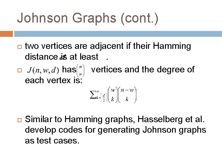
Johnson Graphs (cont. ) two vertices are adjacent if their Hamming distance is at least . has vertices and the degree of each vertex is: Similar to Hamming graphs, Hasselberg et al. develop codes for generating Johnson graphs as test cases.

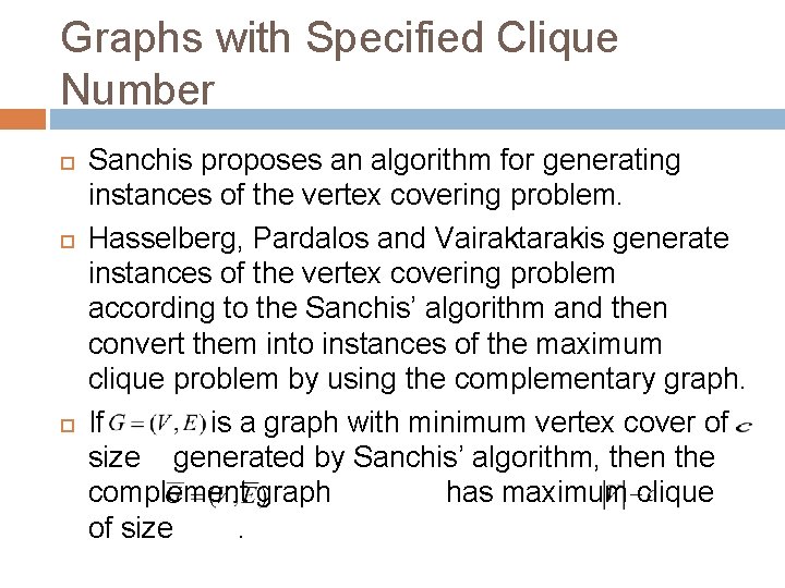
Graphs with Specified Clique Number Sanchis proposes an algorithm for generating instances of the vertex covering problem. Hasselberg, Pardalos and Vairaktarakis generate instances of the vertex covering problem according to the Sanchis’ algorithm and then convert them into instances of the maximum clique problem by using the complementary graph. If is a graph with minimum vertex cover of size generated by Sanchis’ algorithm, then the complement graph has maximum clique of size .

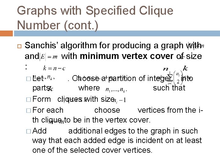
Graphs with Specified Clique Number (cont. ) Sanchis’ algorithm for producing a graph with and with minimum vertex cover of size : � Let . Choose a partition of integer into parts where such that � Form cliques with size � For each choose vertices from the ith clique to be in the vertex cover. � Add additional edges to the graph in such way that each added edge is incident on at least one of the selected cover vertices.

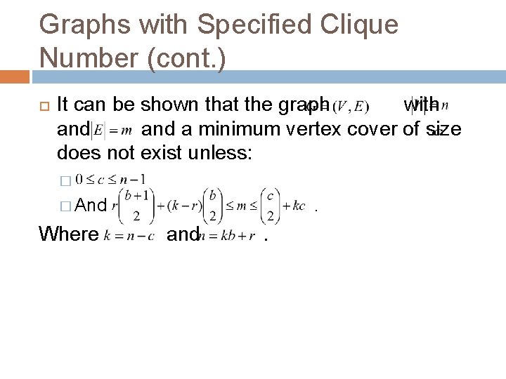
Graphs with Specified Clique Number (cont. ) It can be shown that the graph with and a minimum vertex cover of size does not exist unless: � � And . Where and .

Keller's Conjecture Minkowski's conjecture: � In a lattice tiling of Rn by translates of a unit hypercube, there exists two cubes that share (n 1) dimensional face. � proven by Hajós in 1950 Keller’s conjecture: (1930) � Minkowsk’s theorem can be generalized as the lattice assumption might not be necessary.

Keller's Conjecture (cont. ) Keller’s conjecture: � 1940: Perron showed in 1940 that it true for n ≤ 6 � 1992: Lagarias and Shor found counter-example for n ≥ 10 � 2002: Mackey found counter-example for n ≥ 8 � 2011: n = 7 has been solved Jennifer Debroni, John D. Eblen, Michael A. Langston, Wendy Myrvold, Peter W. Shor, Dinesh Weerapurage. A complete resolution of the Keller maximum clique problem. SODA 2011: 129 -135, 2011

Keller's Conjecture (cont. ) Keller graphs by Corrádi and Szabó: � For any given natural number n, constructed the so-called Keller graph n. The nodes are vectors of length n with values of 0; 1; 2 or 3. Any two vectors are adjacent, if and only if in some of the n coordinates, they differ by precisely two (in absolute value). Properties of Keller Graphs: � Dense graphs where the clique size is bounded by 2 n � There is an counterexample to Keller's conjecture, if and only if n has a clique of size 2 n (Corrádi and

A Comprehensive Survey The most recent survey of results concerning algorithms, complexity, and applications of the maximum clique problem can be found in: � I. M. Bomze, M. Budinich, P. M. Pardalos, and M. Pelillo. The maximum clique problem. In D. -Z. Du and P. M. Pardalos, editors, Handbook of Combinatorial Optimization, pages 1– 74. Kluwer Academic Publishers, Dordrecht, The Netherlands, 1999.

A Comprehensive Survey (cont. ) A complete survey about the graph coloring problem can be found in: � P. M. Pardalos, T. Mavridou, and J. Xue. The Graph coloring problem: A bibliographic survey. In In D. -Z. Du and P. M. Pardalos, editors, Handbook of Combinatorial Optimization, Vol. 2, Pages 331 -396. Kluwer Academic Publishers, Dordrecht, The Netherlands, 1999.

Handbook of Combinatorial Optimization Pardalos, Panos M. ; Du, Ding-Zhu; Graham, Ronald L. (Eds. ) Handbook of Combinatorial Optimization 2 nd ed. 2013, X, 3370 pages, 7 volumes http: //www. springer. com/mathematics/bo ok/978 -1 -4419 -7996 -4

Recent results Mikhail Batsyn, Boris Goldengorin, Evgeny Maslov, Panos M. Pardalos. Improvements to MCS algorithm for the maximum clique problem. Journal of Combinatorial Optimization, DOI 10. 1007/s 10878 -012 -9592 -6, 2013. Abstract. In this paper we present improvements to one of the most recent and fastest branch-and-bound algorithm for the maximum clique problem—MCS algorithm by Tomita et al. (Proceedings of the 4 th international conference on Algorithms and Computation, WALCOM’ 10, pp. 191– 203, 2010). The suggested improvements include: incorporating of an efficient heuristic returning a high-quality initial solution, fast detection of clique vertices in a set of candidates, better initial colouring, and avoiding dynamic memory allocation. Our computational study shows some impressive results, mainly we have solved p_hat 1000 -3 benchmark instance which is intractable for MCS algorithm and got speedups of 7, 3000, and 13000 times for gen 400_p 0. 9_55, gen 400_p 0. 9_65, and gen 400_p 0. 9_75

Recent results Evgeny Maslov, Mikhail Batsyn, Panos M. Pardalos. Speeding up branch and bound algorithms for solving the maximum clique problem. Journal of Global Optimization, DOI 10. 1007/s 10898 -013 -0075 -9, 2013 Abstract In this paper we consider two branch and bound algorithms for the maximum clique problem which demonstrate the best performance on DIMACS instances among the existing methods. These algorithms are MCS algorithm by Tomita et al. (2010) and MAXSAT algorithm by Li and Quan (2010 a, b). We suggest a general approach which allows us to speed up considerably these branch and bound algorithms on hard instances. The idea is to apply a powerful heuristic for obtaining an initial solution of high quality. This solution is then used to prune branches in the main branch and bound algorithm. For this purpose we apply ILS heuristic by Andrade et al. (J Heuristics 18(4): 525– 547, 2012). The best results are obtained for p_hat 1000 -3 instance and gen instances with up to 11, 000 times speedup.