Computational Biology Lecture 10 Analyzing Gene Expression Data

Computational Biology Lecture #10: Analyzing Gene Expression Data Bud Mishra Professor of Computer Science and Mathematics 11 ¦ 26 ¦ 2001 9/25/2020 ©Bud Mishra, 2001 1

The Computational Tasks • Clustering Genes: – Which genes are regulated together? • Classifying Genes: – Which functional class does a particular gene fall into? • Classifying Gene Expressions: – What can be learnt about a cell from the set of all m. RNA expressed in a cell? Classifying diseases: Does a patient have ALL or AML (classes of Leukemia)? • Inferring Regulatory Networks: – What is the “circuitry” of the cell? 9/25/2020 ©Bud Mishra, 2001 2

Support Vector Machine • Classification Microarray Expression Data • Brown, Grundy, Lin, Cristianini, Sugnet, Ares & Haussler ’ 99 • Analysis of S. cerevisiae data from Pat Brown’s Lab (Stanford) – Instead of clustering genes to see what groupings emerge – Devise models to match genes to predefined classes 9/25/2020 ©Bud Mishra, 2001 3

The Data • 79 measurements for each of 2467 genes • Data collected at various times during – Diauxic shift (shutting down genes for metabolizing sugar, activating genes for metabolizing ethanol) – Mitotic cell division cycle – Sporulation – Temperature shock – Reducing Shock 9/25/2020 ©Bud Mishra, 2001 4

Genome-wide Cluster Analysis • Each measurement Gi represents log (redi/greeni) Where red is the test expression level and green is the reference expression level for gene G in the ith experiment. • The expression profile of a gene is the vector of measurements across all experiments: h G 1, …, Gm i. 9/25/2020 ©Bud Mishra, 2001 5

The Data • n genes measured in m experiments: Vector for a gene G 1, 1 L G 1, n G 2, 1 L G 2, n M O M Gm, 1 L Gm, n Class 1 9/25/2020 Classn ©Bud Mishra, 2001 6

The Classes • From the MIPS yeast genome database (MYGD) – – – Tricarboxylic acid pathway (Krebs cycle) Respiration chain complexes Cytoplasmic riosomal potins Proteasome Histones Helix-turn-helix (control) • Classes come from biochemical/genetic studies of genes 9/25/2020 ©Bud Mishra, 2001 7

Gene Classification • Learning Task – Given: Expression profiles of genes and their class tables – Do: Learn models distinguishing genes of each class from genes in other classes • Classification Task – Given: Expression profile of a gene whose class is not unknown – Do: Predict the class to which this gene belongs 9/25/2020 ©Bud Mishra, 2001 8

The Approach • Brown et al. applies a variety of algorithms to this task: – Support vector machines (SVMs) [Vapnik ’ 95] – Decision Trees – Parzen Windows – Fisher linear discriminant 9/25/2020 ©Bud Mishra, 2001 9

Support Vector Machines Experiment 2 • Consider the genes in our example as m points in an ndimensional space (m genes, n experiments) Experiment 1 9/25/2020 ©Bud Mishra, 2001 10

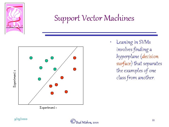
Support Vector Machines Experiment 2 • Leaning in SVMs involves finding a hyperplane (decision surface) that separates the examples of one class from another. Experiment 1 9/25/2020 ©Bud Mishra, 2001 11

Support Vector Machines • For the ith example, let xi be the vector of expression measurements, and yi be +1, if the example is in the class of interest; and – 1, otherwise • The hyperplane is given by: w¢x+b=0 where b = constant and w= vector of weights 9/25/2020 ©Bud Mishra, 2001 12

Support Vector Machines • The function used to classify examples is then y. P = sgn(w ¢ x + b) where y. P = predicted value of y. 9/25/2020 ©Bud Mishra, 2001 13

Support Vector Machines Experiment 2 • There may be many such hyperplanes. . • Which one should we choose? Experiment 1 9/25/2020 ©Bud Mishra, 2001 14

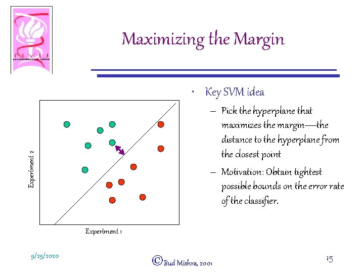
Maximizing the Margin • Key SVM idea Experiment 2 – Pick the hyperplane that maximizes the margin—the distance to the hyperplane from the closest point – Motivation: Obtain tightest possible bounds on the error rate of the classifier. Experiment 1 9/25/2020 ©Bud Mishra, 2001 15

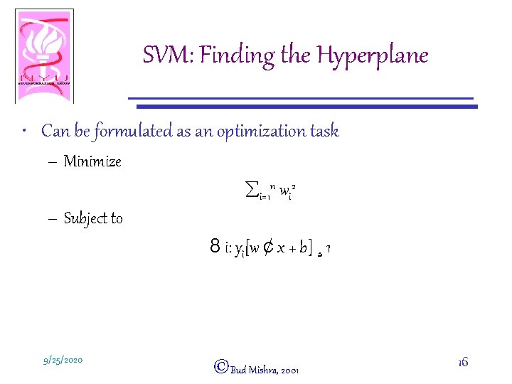
SVM: Finding the Hyperplane • Can be formulated as an optimization task – Minimize åi=1 n wi 2 – Subject to 8 i: yi[w ¢ x + b] ¸ 1 9/25/2020 ©Bud Mishra, 2001 16

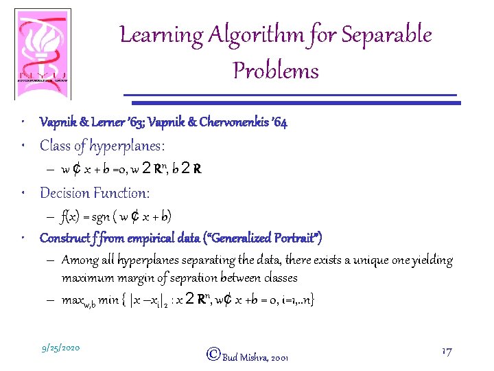
Learning Algorithm for Separable Problems • Vapnik & Lerner ’ 63; Vapnik & Chervonenkis ’ 64 • Class of hyperplanes: – w ¢ x + b =0, w 2 Rn, b 2 R • Decision Function: – f(x) = sgn ( w ¢ x + b) • Construct f from empirical data (“Generalized Portrait”) – Among all hyperplanes separating the data, there exists a unique one yielding maximum margin of sepration between classes – maxw, b min { |x –xi|2 : x 2 Rn, w¢ x +b = 0, i=1, . . n} 9/25/2020 ©Bud Mishra, 2001 17

Maximum Margin x 1 x 2 {x | w¢ x + b = +1} w w ¢ x 1 + b = +1 w ¢ x 2 + b = -1 {x | w¢ x + b = 0} ) (x 1 - x 2) 1 w = 2 /|w|2 {x | w¢ x + b = -1} 9/25/2020 w ¢ (x 1 – x 2) = 2 ©Bud Mishra, 2001 18

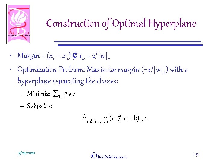
Construction of Optimal Hyperplane • Margin = (x 1 – x 2) ¢ 1 w = 2/|w|2 • Optimization Problem: Maximize margin (=2/|w|2) with a hyperplane separating the classes: – Minimize åi=1 m wi 2 – Subject to 8 i 2 {1, . . n} yi (w ¢ xi + b) ¸ 1. 9/25/2020 ©Bud Mishra, 2001 19

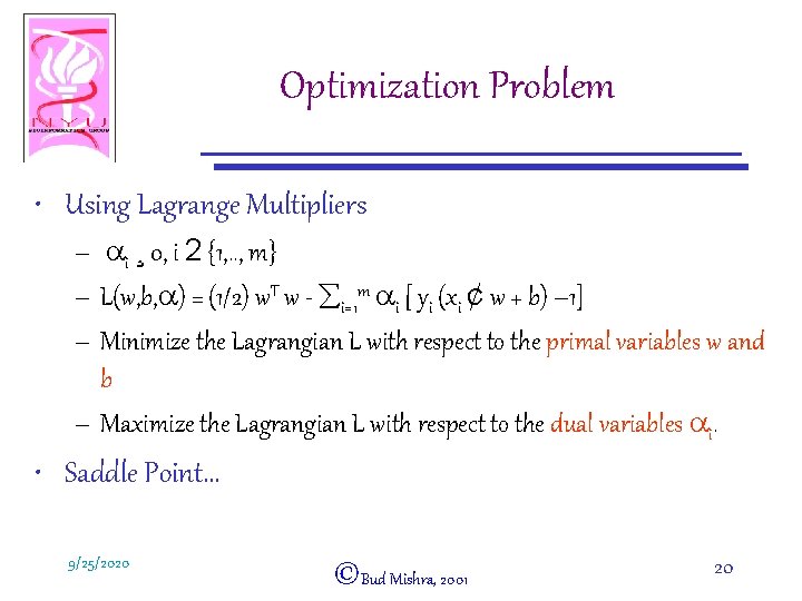
Optimization Problem • Using Lagrange Multipliers – ai ¸ 0, i 2 {1, . . , m} – L(w, b, a) = (1/2) w. T w - åi=1 m ai [ yi (xi ¢ w + b) – 1] – Minimize the Lagrangian L with respect to the primal variables w and b – Maximize the Lagrangian L with respect to the dual variables ai. • Saddle Point… 9/25/2020 ©Bud Mishra, 2001 20

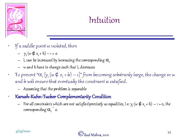
Intuition • If a saddle point is violated, then – yi (w ¢ xi + b) – 1 < 0 – L can be increased by increasing the corresponding ai – w and b have to change such that L decreases • To prevent “ai [yi (w ¢ xi + b) – 1]” from becoming arbitrarily large, the change in w and b will ensure that eventually the constraint is satisfied. – Assuming that the problem is separable • Karush-Kuhn-Tucker Complementarity Condition – For all constraints which are not satisfied precisely as equalities, I. e. yi (w ¢ xi + b) – 1 > 0, the corresponding a. I ´ 0. 9/25/2020 ©Bud Mishra, 2001 21

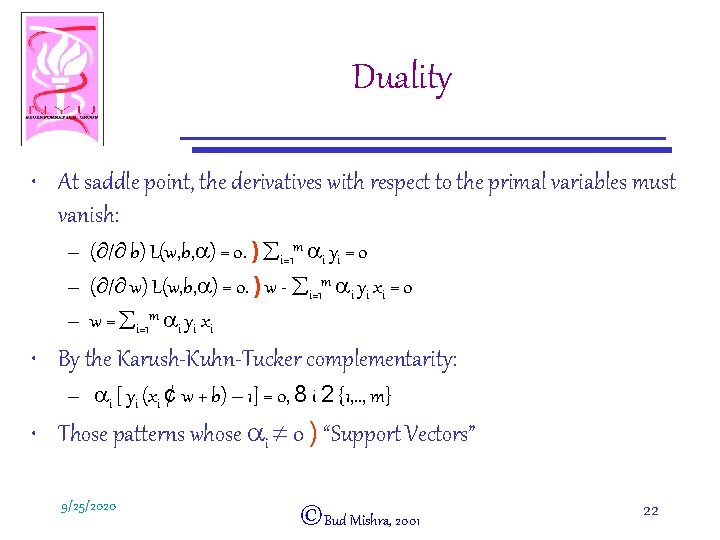
Duality • At saddle point, the derivatives with respect to the primal variables must vanish: – (¶/¶ b) L(w, b, a) = 0. ) åi=1 m ai yi = 0 – (¶/¶ w) L(w, b, a) = 0. ) w - åi=1 m ai yi xi = 0 – w = åi=1 m ai yi xi • By the Karush-Kuhn-Tucker complementarity: – ai [ yi (xi ¢ w + b) – 1] = 0, 8 i 2 {1, . . , m} • Those patterns whose ai ¹ 0 ) “Support Vectors” 9/25/2020 ©Bud Mishra, 2001 22

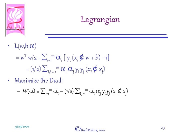
Lagrangian • L(w, b, a) = w. T w/2 - åi=1 m ai [ yi (xi ¢ w + b) – 1] = (1/2) åi, j = 1 m ai aj y. I yj (xi ¢ xj) • Maximize the Dual: – W(a) = åi=1 m ai – (1/2) åi, j=1 m ai aj yi yj (xi ¢ xj) 9/25/2020 ©Bud Mishra, 2001 23

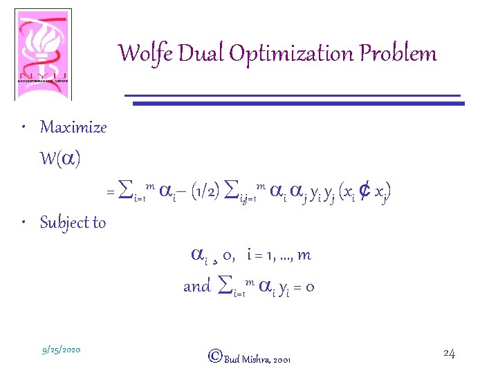
Wolfe Dual Optimization Problem • Maximize W(a) = åi=1 m ai– (1/2) åi, j=1 m ai aj yi yj (xi ¢ xj) • Subject to ai ¸ 0, i = 1, …, m and åi=1 m ai yi = 0 9/25/2020 ©Bud Mishra, 2001 24

Decision Function • The hyperplane decision function can be written as f(x) = sgn( åi=1 m yi ai (x ¢ xi) + b] • Where b is the solytion to ai [ yi (xi ¢ w + b) – 1] = 0 9/25/2020 ©Bud Mishra, 2001 25

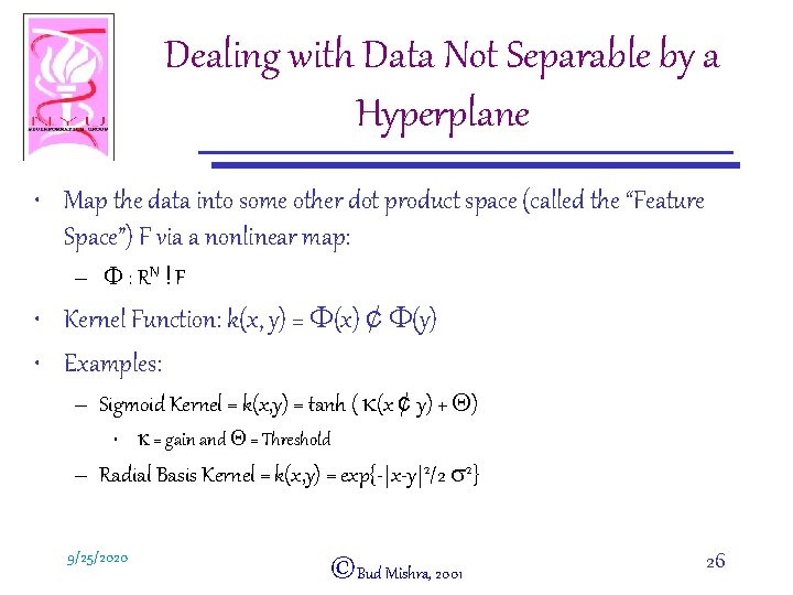
Dealing with Data Not Separable by a Hyperplane • Map the data into some other dot product space (called the “Feature Space”) F via a nonlinear map: – F : RN ! F • Kernel Function: k(x, y) = F(x) ¢ F(y) • Examples: – Sigmoid Kernel = k(x, y) = tanh ( k(x ¢ y) + Q) • k = gain and Q = Threshold – Radial Basis Kernel = k(x, y) = exp{-|x-y|2/2 s 2} 9/25/2020 ©Bud Mishra, 2001 26

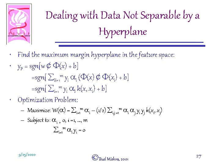
Dealing with Data Not Separable by a Hyperplane • Find the maximum margin hyperplane in the feature space: • y. P = sgn[w ¢ F(x) + b] =sgn[ åIi=1 m yi ai (F(x) ¢ F(xi) + b] =sgn[ åi=1 m yi a. I k(x, xi) + b] • Optimization Problem: – Maximize: W(a) = åi=1 m ai – (1/2) åi, j =1 m ai aj yi yj k(xi, xj) – Subject to: ai ¸ 0, i =1, …, m åi=1 m ai yi = 0 9/25/2020 ©Bud Mishra, 2001 27

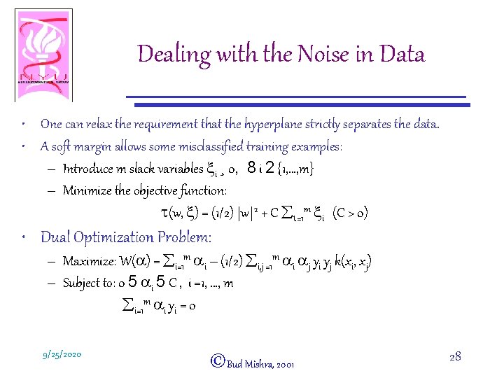
Dealing with the Noise in Data • One can relax the requirement that the hyperplane strictly separates the data. • A soft margin allows some misclassified training examples: – Introduce m slack variables xi ¸ 0, 8 i 2 {1, …, m} – Minimize the objective function: t(w, x) = (1/2) |w|2 + C åi=1 m xi (C > 0) • Dual Optimization Problem: – Maximize: W(a) = åi=1 m ai – (1/2) åi, j =1 m ai aj yi yj k(xi, xj) – Subject to: 0 5 ai 5 C , i =1, …, m åi=1 m ai yi = 0 9/25/2020 ©Bud Mishra, 2001 28

SVM & Neural Networks • SVM • Neural Network – Represents linear or nonlinear separating surface – Weights determined by optimization method (optimizing margins) 9/25/2020 – Represents linear or nonlinear separating surface – Weights determined by optimization method (optimizing sum of squared error—or a related objective function) ©Bud Mishra, 2001 29

Experiments • 3 -fold cross validation • Create a separate model for each class • SVM with various kernel functions – Dot product raised to power d= 1, 2, 3: k(x, y) = (x¢ y)d – Gaussian • Various Other Classification Methods – Decision trees – Parzen windows – Fisher linear discriminant 9/25/2020 ©Bud Mishra, 2001 30

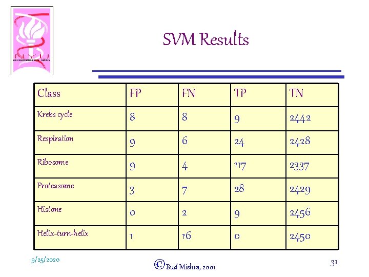
SVM Results Class FP FN TP TN Krebs cycle 8 8 9 2442 Respiration 9 6 24 2428 Ribosome 9 4 117 2337 Proteasome 3 7 28 2429 Histone 0 2 9 2456 Helix-turn-helix 1 16 0 2450 9/25/2020 ©Bud Mishra, 2001 31

SVM Results • SVM had highest accuracy for all classes (except the control) • Many of the false positives could be easily explained in terms of the underlying biology: – E. g. YAL 003 W was repeatedly assigned to the ribosome class • Not a ribosomal protein • But known to be required for proper functioning of the ribosome. 9/25/2020 ©Bud Mishra, 2001 32