Compressing Polygon Mesh Geometry with Parallelogram Prediction Martin

Compressing Polygon Mesh Geometry with Parallelogram Prediction Martin Isenburg Pierre Alliez UNC Chapel Hill INRIA Sophia-Antipolis

Take this home: “Non-triangular faces in the mesh can be exploited for more efficient predictive compression of vertex positions. ” “Non-triangular faces tend to be planar and convex. ”

Overview • • Background Previous Work Linear Prediction Schemes “within” versus “across” Example Run Can we do better ? Conclusion

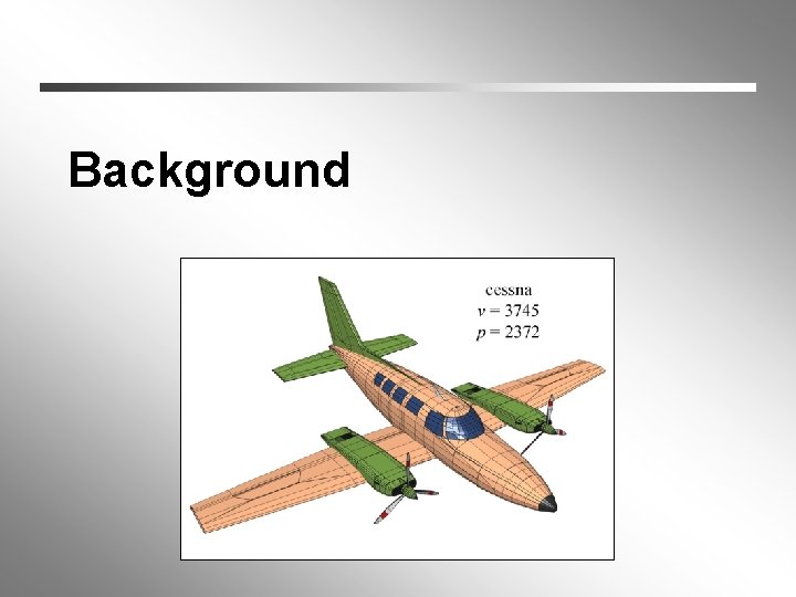
Background

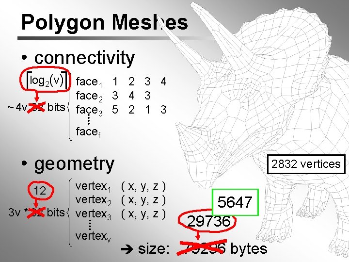
Polygon Meshes • connectivity log 2(v) face 1 1 2 3 4 face 2 3 4 3 ~ 4 v 32 bits face 3 5 2 1 3 facef • geometry 2832 vertices vertex 1 ( x, y, z ) vertex 2 ( x, y, z ) 3 v * 32 bits vertex 3 ( x, y, z ) 12 vertexv 5647 29736 size: 79296 bytes

Mesh Compression • Geometry Compression [[Deering, 95] – Fast Rendering – Progressive Transmission – Maximum. Compression

Mesh Compression • Geometry Compression [[Deering, 95] – Fast Rendering – Progressive Transmission – Maximum. Compression • Connectivity • Geometry

Mesh Compression • Geometry Compression [[Deering, 95] – Fast Rendering – Progressive Transmission – Maximum. Compression • Connectivity • Geometry – Triangle Meshes – Polygon. Meshes

Triangle Mesh Compression [Touma & Gotsman, Graphics Interface 98] • Connectivity Coder – stores the connectivity as sequence of vertex degrees • Geometry Coder – stores the geometry as sequence of vectors; each corrects the prediction of a vertex position

Not Triangles … Polygons! Face Fixer [Isenburg & Snoeyink, 00]

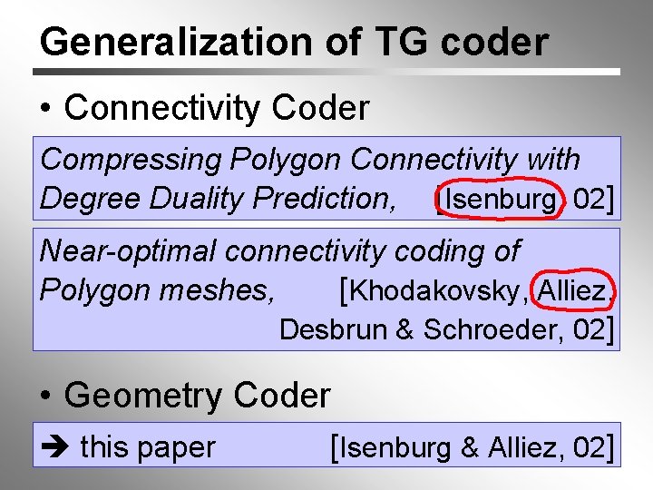
Generalization of TG coder • Connectivity Coder Compressing Polygon Connectivity with Degree Duality Prediction, [Isenburg, 02] Near-optimal connectivity coding of Polygon meshes, [Khodakovsky, Alliez, Desbrun & Schroeder, 02] • Geometry Coder this paper [Isenburg & Alliez, 02]

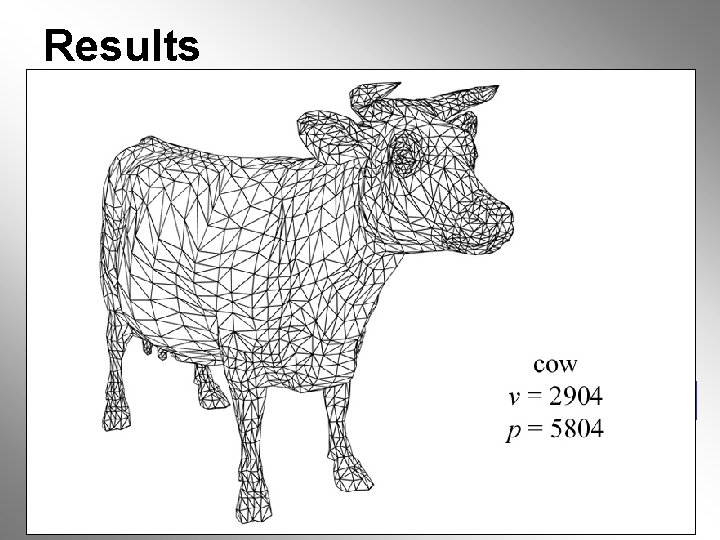
Results bits per vertex model TG IA gain triceratops galleon cessna … tommygun cow teapot 20. 0 24. 1 19. 1 14. 8 18. 4 12. 5 26 % 35 %. . . 36 % -1 % 24 % … … 19. 6 20. 4 21. 0 12. 5 20. 6 16. 1 min / max / average [%] = 9 / 41 / 23

Previous Work

Previous Work • Classic approaches [95 – 98]: – linear prediction Geometry Compression Java 3 D [Deering, 95] Geometric Compression through topological surgery [Taubin & Rossignac, 98] MPEG - 4 Triangle Mesh Compression Virtue 3 D [Touma & Gotsman, 98]

Previous Work • Classic approaches [95 – 98]: – linear prediction • Recent approaches [00 – 02]: – – – spectral re-meshing space-dividing vector-quantization feature discovery angle-based

Previous Work • Classic approaches [95 – 98]: – linear prediction • Recent approaches [00 – 02]: – – – spectral Spectral Compression of Mesh Geometry re-meshing [Karni & Gotsman, 00] space-dividing vector-quantization feature discovery expensive numerical computations angle-based

Previous Work • Classic approaches [95 – 98]: – linear prediction • Recent approaches [00 – 02]: – – – spectral Progressive Geometry Compression re-meshing [Khodakovsky et al. , 00] space-dividing vector-quantization feature discovery modifies mesh prior to compression angle-based

Previous Work • Classic approaches [95 – 98]: – linear prediction • Recent approaches [00 – 02]: – – – spectral Geometric Compression for interactive transmission re-meshing [Devillers & Gandoin, 00] space-dividing vector-quantization feature discovery poly-soups; complex geometric algorithms angle-based

Previous Work • Classic approaches [95 – 98]: – linear prediction • Recent approaches [00 – 02]: – – – spectral Vertex data compression for triangle meshes re-meshing [Lee & Ko, 00] space-dividing vector-quantization feature discovery local coord-system + vector-quantization angle-based

Previous Work • Classic approaches [95 – 98]: – linear prediction • Recent approaches [00 – 02]: – – – spectral Compression of engineering models by repeated feature re-meshing discovery [Shikhare et al. , 01] space-dividing vector-quantization feature discovery certain 3 D models + expensive matching angle-based

Previous Work • Classic approaches [95 – 98]: – linear prediction • Recent approaches [00 – 02]: – – – spectral Angle-Analyzer: A trianglequad mesh codec re-meshing [Lee, Alliez & Desbrun, 02] space-dividing vector-quantization feature discovery dihedral + internal = heavy trigonometry angle-based

Linear Prediction Schemes

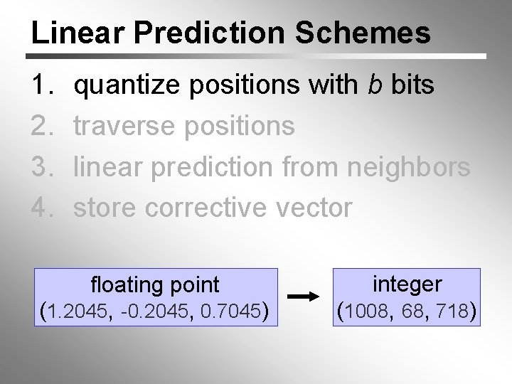
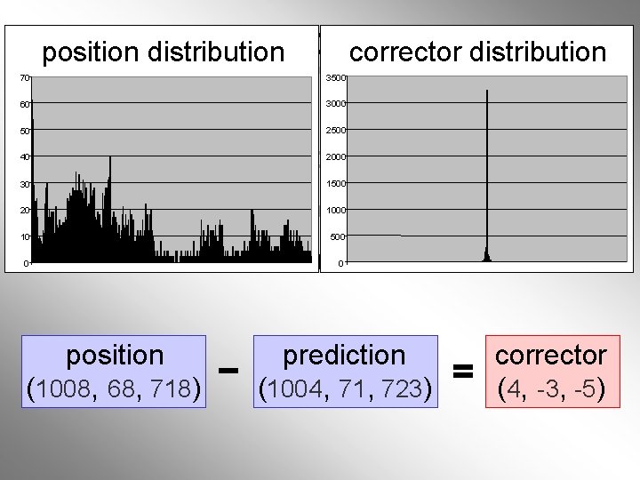
Linear Prediction Schemes 1. 2. 3. 4. quantize positions with b bits traverse positions linear prediction from neighbors store corrective vector floating point (1. 2045, -0. 2045, 0. 7045) integer (1008, 68, 718)

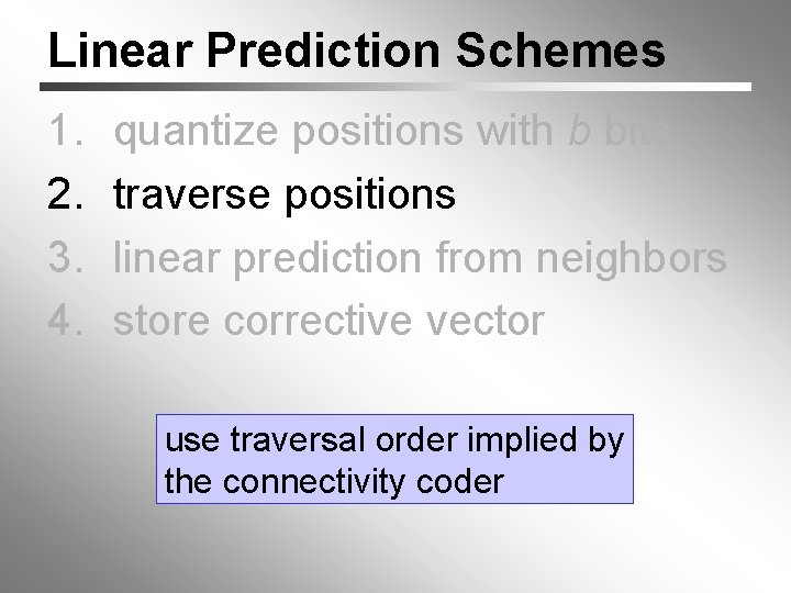
Linear Prediction Schemes 1. 2. 3. 4. quantize positions with b bits traverse positions linear prediction from neighbors store corrective vector use traversal order implied by the connectivity coder

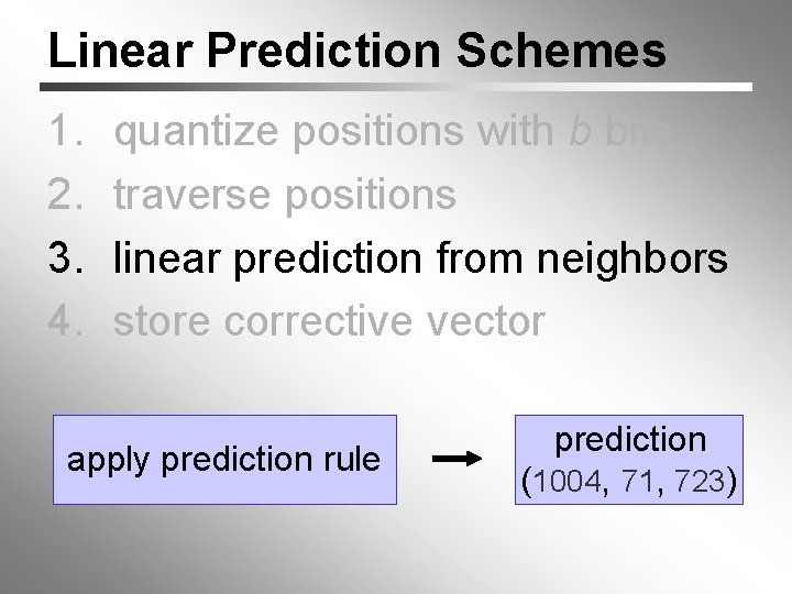
Linear Prediction Schemes 1. 2. 3. 4. quantize positions with b bits traverse positions linear prediction from neighbors store corrective vector apply prediction rule prediction (1004, 71, 723)

Linear Predictioncorrector Schemes position distribution 3500 70 60 50 40 30 20 10 0 1. 2. 3. 4. quantize positions with b bits traverse positions linear prediction from neighbors store corrective vector position (1008, 68, 718) 3000 2500 2000 1500 1000 500 0 prediction (1004, 71, 723) corrector (4, -3, -5)

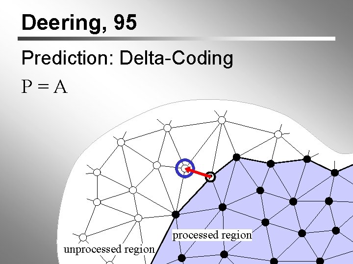
Deering, 95 Prediction: Delta-Coding P=A P A processed region unprocessed region

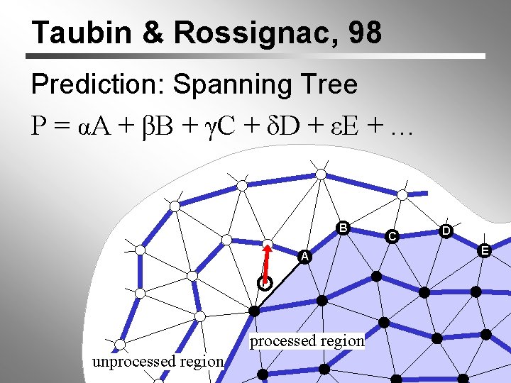
Taubin & Rossignac, 98 Prediction: Spanning Tree P = αA + βB + γC + δD + εE + … B A P processed region unprocessed region C D E

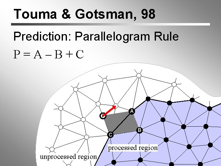
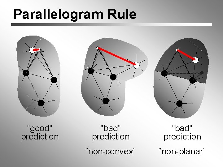
Touma & Gotsman, 98 Prediction: Parallelogram Rule P=A–B+C A P C B processed region unprocessed region

Parallelogram Rule “good” prediction “bad” prediction “non-convex” “non-planar”

More “good” Predictions Multi-way geometry encoding. [Cohen-Or, Cohen & Irony, 02] • average multiple predictions average gain of 11 % Optimized compression of triangle mesh geometry using prediction trees. [Kronrod & Gotsman, 02] • search for best prediction • direct the traversal (prediction tree) average gain of 8 % (smooth) & 42 % (CAD)

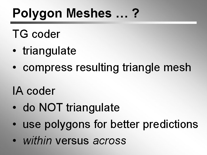
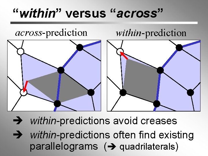
Polygon Meshes … ? TG coder • triangulate • compress resulting triangle mesh IA coder • do NOT triangulate • use polygons for better predictions • within versus across

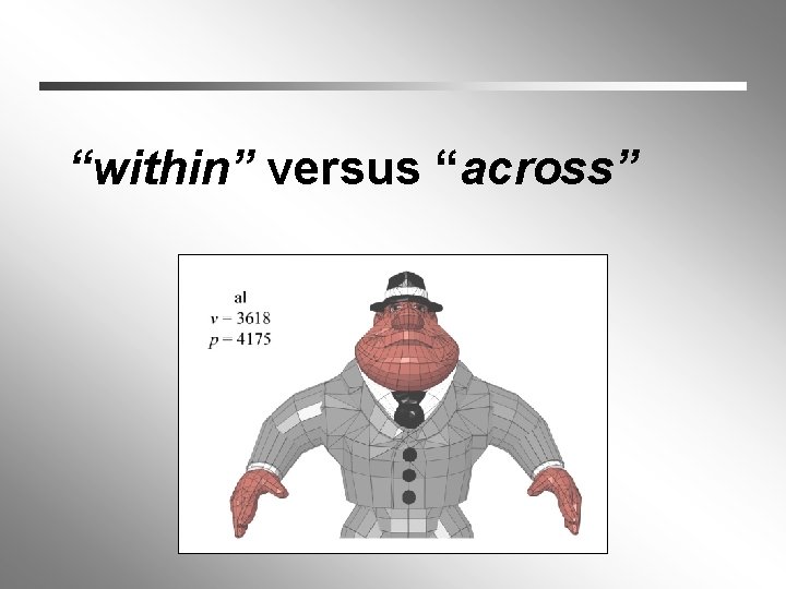
“within” versus “across”

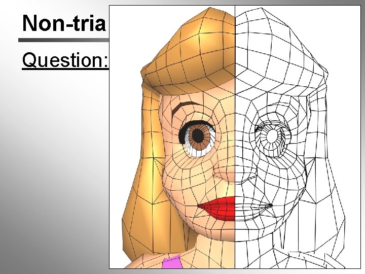
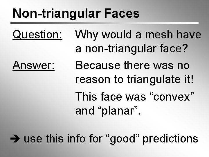
Non-triangular Faces Question: Why would a mesh have a non-triangular face?

Non-triangular Faces Question: Answer: Why would a mesh have a non-triangular face? Because there was no reason to triangulate it! This face was “convex” and “planar”. use this info for “good” predictions

“within” versus “across” across-prediction within-predictions avoid creases within-predictions often find existing parallelograms ( quadrilaterals)

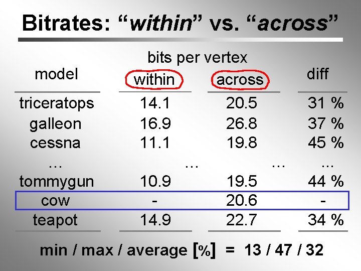
Bitrates: “within” vs. “across” model triceratops galleon cessna … tommygun cow teapot bits per vertex within across 20. 5 14. 1 26. 8 16. 9 19. 8 11. 1 … … 19. 5 10. 9 20. 6 22. 7 14. 9 diff 31 % 37 % 45 %. . . 44 % 34 % min / max / average [%] = 13 / 47 / 32

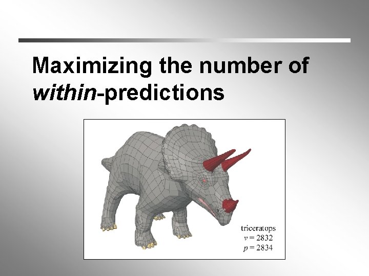
Maximizing the number of within-predictions

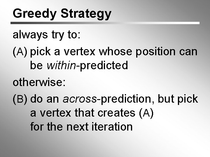
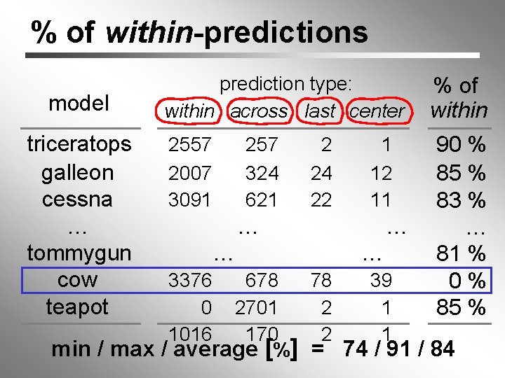
Greedy Strategy always try to: (A) pick a vertex whose position can be within-predicted otherwise: (B) do an across-prediction, but pick a vertex that creates (A) for the next iteration

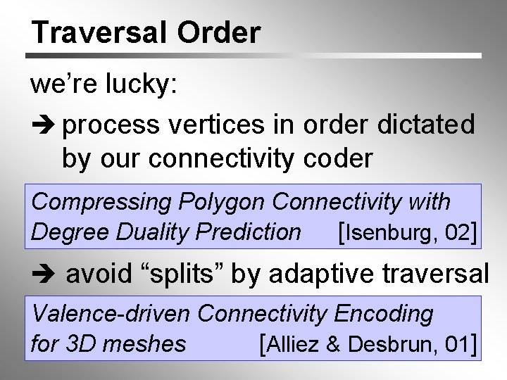
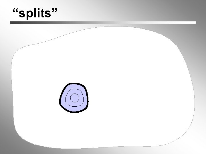
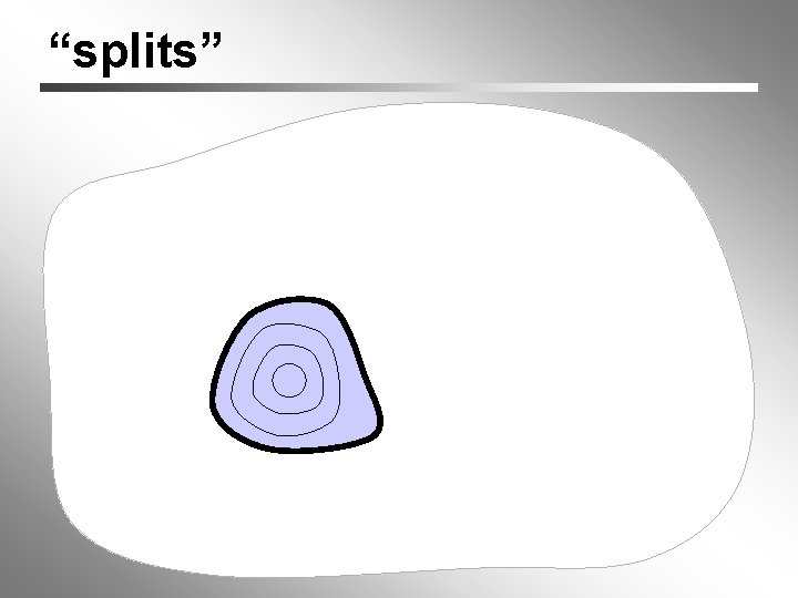
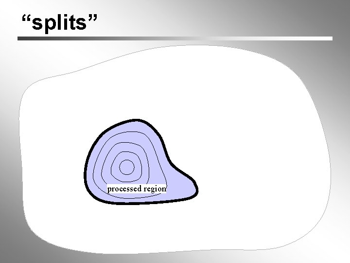
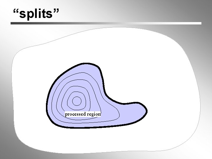
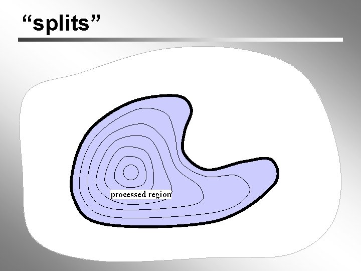
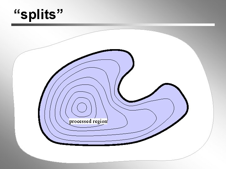
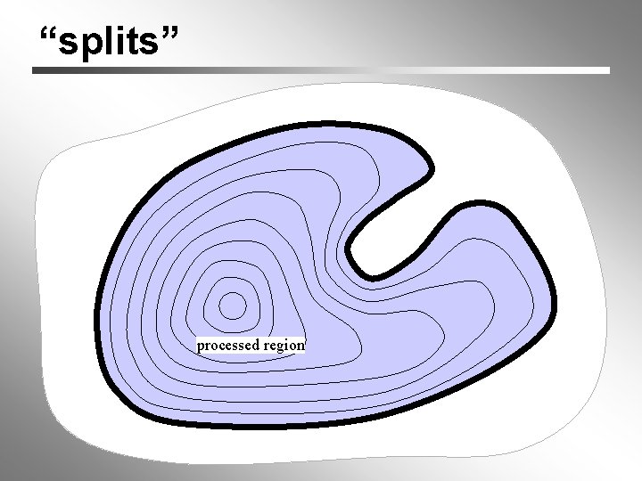
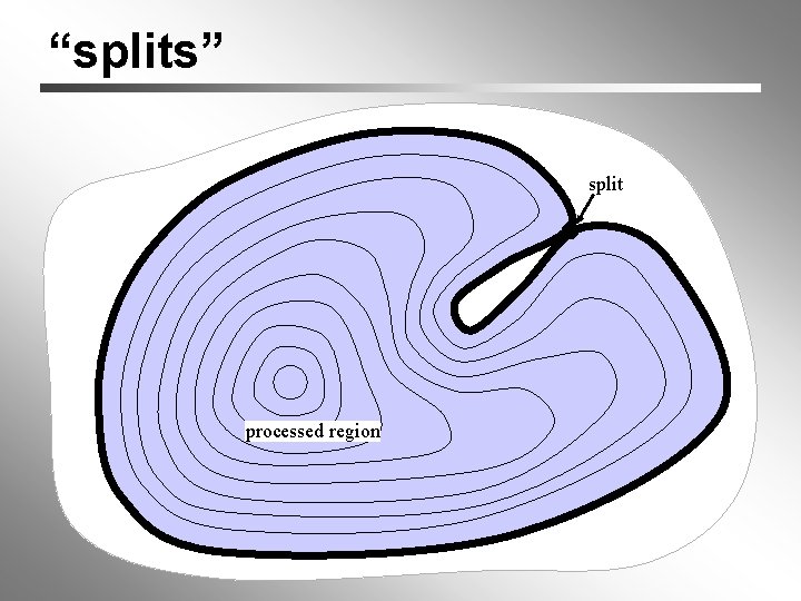
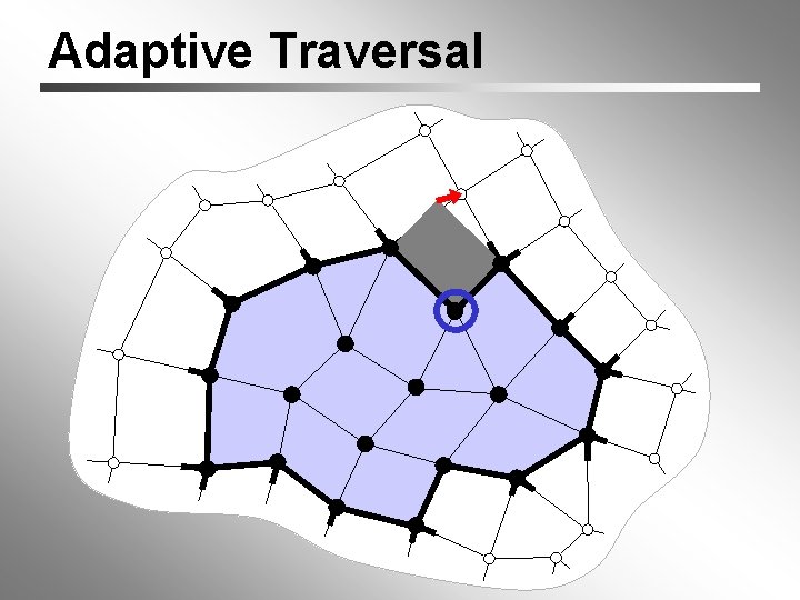
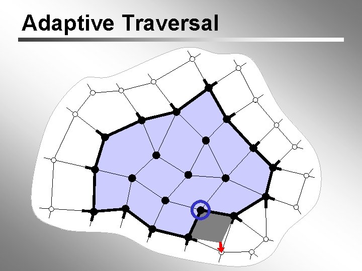
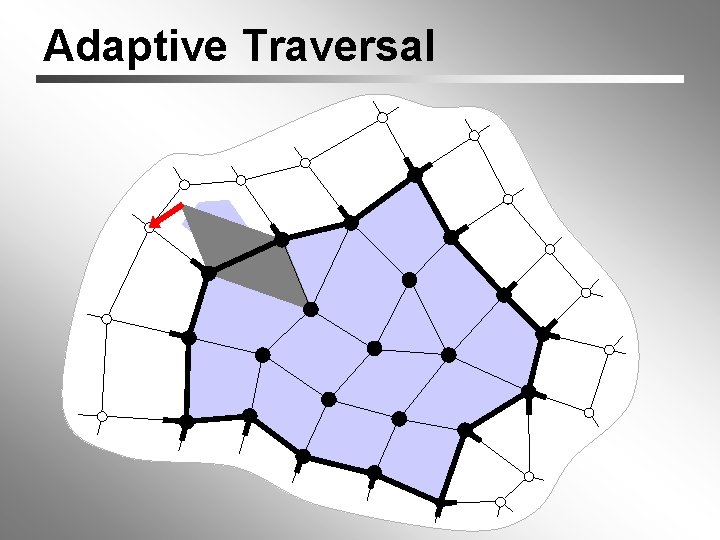
Traversal Order we’re lucky: process vertices in order dictated by our connectivity coder Compressing Polygon Connectivity with Degree Duality Prediction [Isenburg, 02] avoid “splits” by adaptive traversal Valence-driven Connectivity Encoding for 3 D meshes [Alliez & Desbrun, 01]

“splits”

“splits”

“splits”

“splits”

“splits” processed region

“splits” processed region

“splits” processed region

“splits” processed region

“splits” processed region

“splits” split processed region

Adaptive Traversal

Adaptive Traversal

Adaptive Traversal

% of within-predictions model triceratops galleon cessna … tommygun cow teapot prediction type: within across last center 2557 2007 3091 257 324 621 2 24 22 1 12 11 … … 3376 0 1016 … … % of within 90 % 85 % 83 % … 81 % 0% 85 % 678 78 39 2701 2 1 170 2 1 min / max / average [%] = 74 / 91 / 84

Example Decoding Run

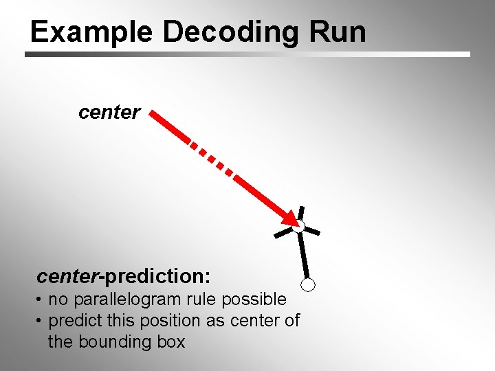
Example Decoding Run center-prediction: • no parallelogram rule possible • predict this position as center of the bounding box

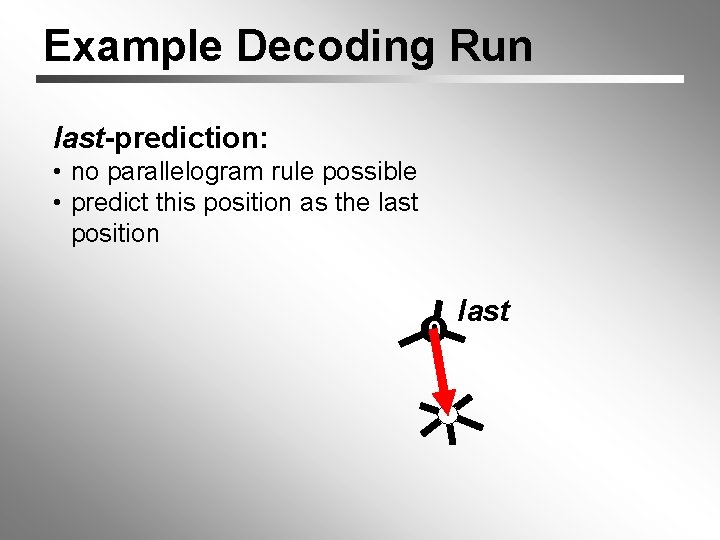
Example Decoding Run last-prediction: • no parallelogram rule possible • predict this position as the last position 0 last

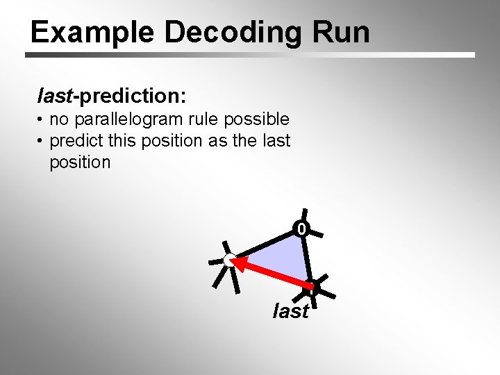
Example Decoding Run last-prediction: • no parallelogram rule possible • predict this position as the last position 0 1 last

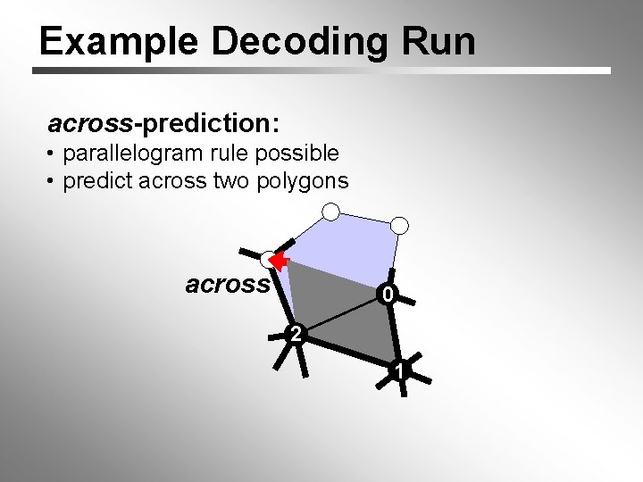
Example Decoding Run across-prediction: • parallelogram rule possible • predict across two polygons across 0 2 1

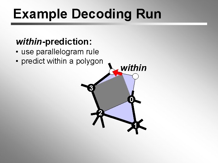
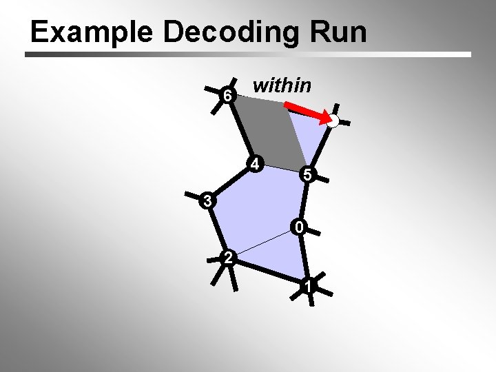
Example Decoding Run within-prediction: • use parallelogram rule • predict within a polygon within 3 0 2 1

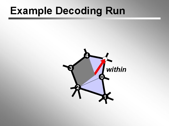
Example Decoding Run 4 3 within 0 2 1

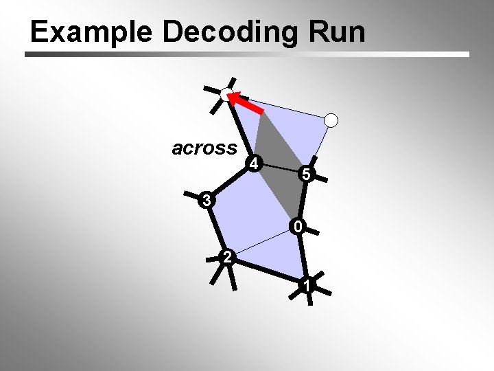
Example Decoding Run across 4 5 3 0 2 1

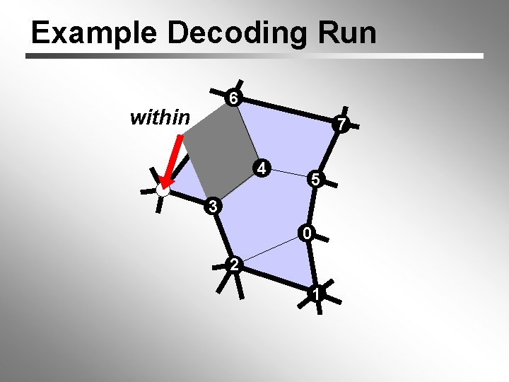
Example Decoding Run 6 within 4 5 3 0 2 1

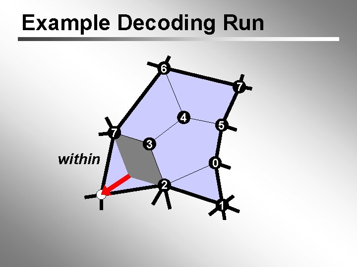
Example Decoding Run 6 within 7 4 5 3 0 2 1

Example Decoding Run 6 7 4 7 within 5 3 0 2 1

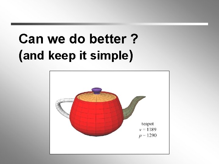
Can we do better ? (and keep it simple)

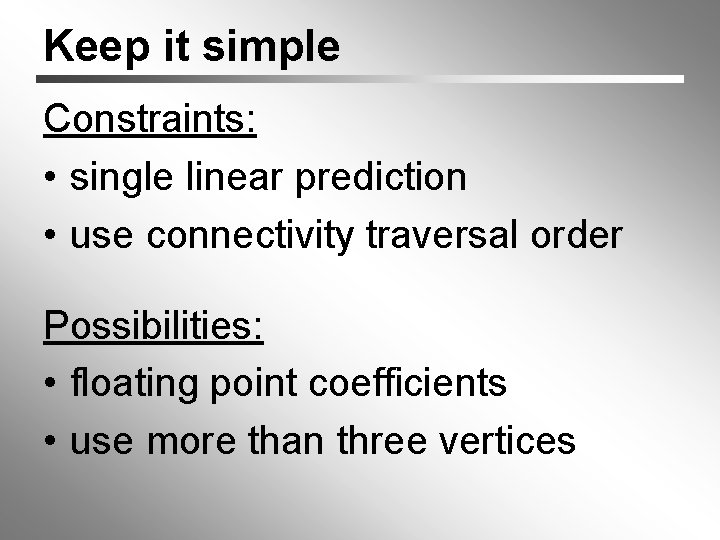
Keep it simple Constraints: • single linear prediction • use connectivity traversal order Possibilities: • floating point coefficients • use more than three vertices

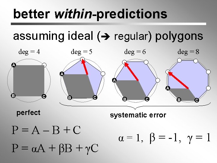
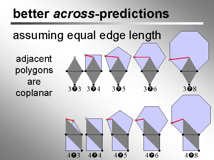
better within-predictions assuming ideal ( regular) polygons deg = 5 deg = 4 deg = 8 deg = 6 A A B C perfect P=A–B+C P = αA + βB + γC B C systematic error α = 1, β = -1, γ = 1

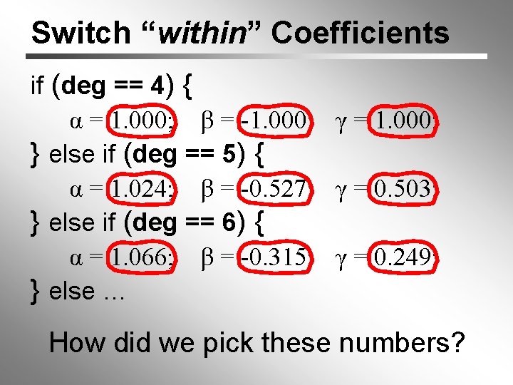
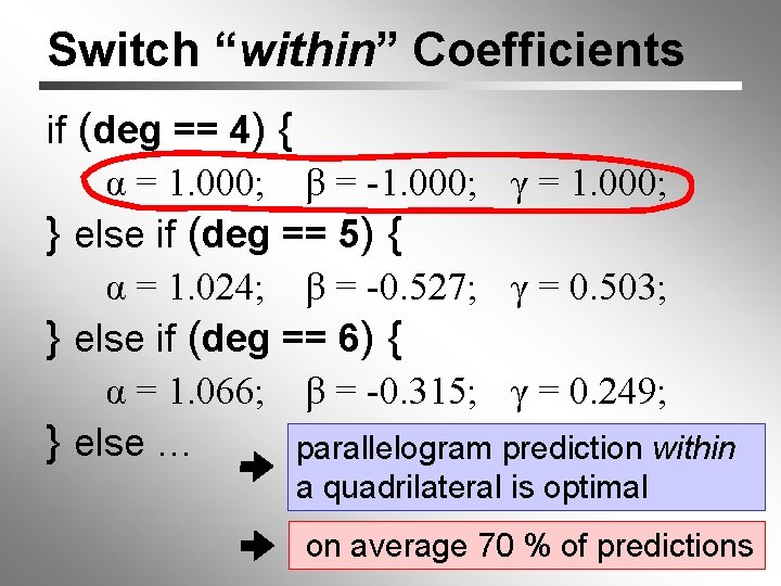
Switch “within” Coefficients if (deg == 4) { α = 1. 000; β = -1. 000; γ = 1. 000; } else if (deg == 5) { α = 1. 024; β = -0. 527; γ = 0. 503; } else if (deg == 6) { α = 1. 066; β = -0. 315; γ = 0. 249; } else … How did we pick these numbers?

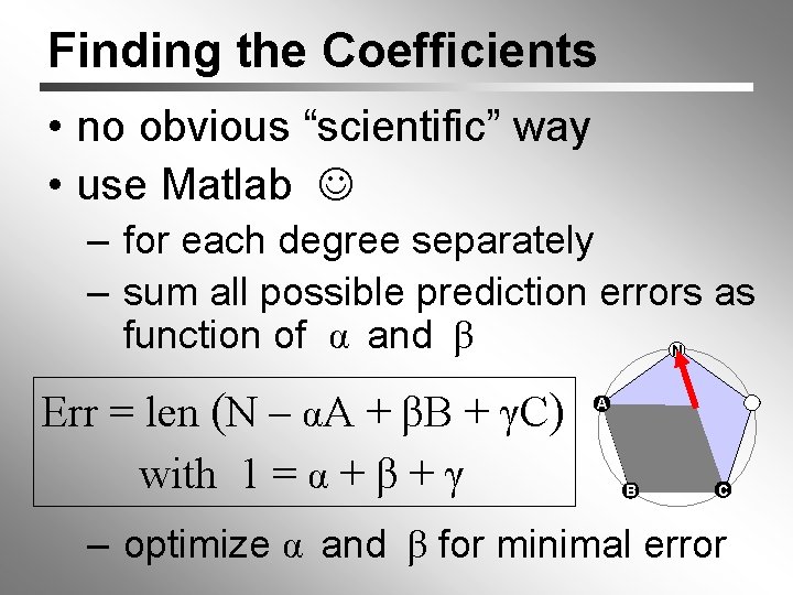
Finding the Coefficients • no obvious “scientific” way • use Matlab – for each degree separately – sum all possible prediction errors as function of α and β N Err = len (N – αA + βB + γC) with 1 = α + β + γ A B C – optimize α and β for minimal error

Switch “within” Coefficients if (deg == 4) { α = 1. 000; β = -1. 000; γ = 1. 000; } else if (deg == 5) { α = 1. 024; β = -0. 527; γ = 0. 503; } else if (deg == 6) { α = 1. 066; β = -0. 315; γ = 0. 249; } else … parallelogram prediction within a quadrilateral is optimal on average 70 % of predictions

better across-predictions assuming equal edge length adjacent polygons are coplanar 3 3 3 4 3 5 3 6 3 8 4 3 4 5 4 6 4 8 4 4

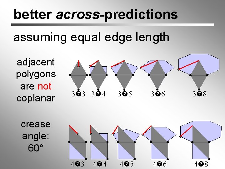
better across-predictions assuming equal edge length adjacent polygons are not coplanar 3 3 3 4 3 5 3 6 3 8 4 3 4 5 4 6 4 8 crease angle: 60° 4 4

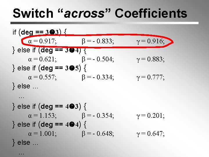
Switch “across” Coefficients if (deg == 3 3) { α = 0. 917; β = - 0. 833; } else if (deg == 3 4) { α = 0. 621; β = - 0. 504; } else if (deg == 3 5) { α = 0. 557; β = - 0. 334; } else … … γ = 0. 916; γ = 0. 883; γ = 0. 777; } else if (deg == 4 3) { α = 1. 153; β = - 0. 354; } else if (deg == 4 4) { α = 1. 001; β = - 0. 648; } else … … γ = 0. 201; γ = 0. 647;

Conclusion

Summary (1) • polygon information can improve predictive geometry compression • using parallelogram rule “within” rather than “across” polygons • average improvement of 23 % over TG coder • has simple and straight-forward implementation

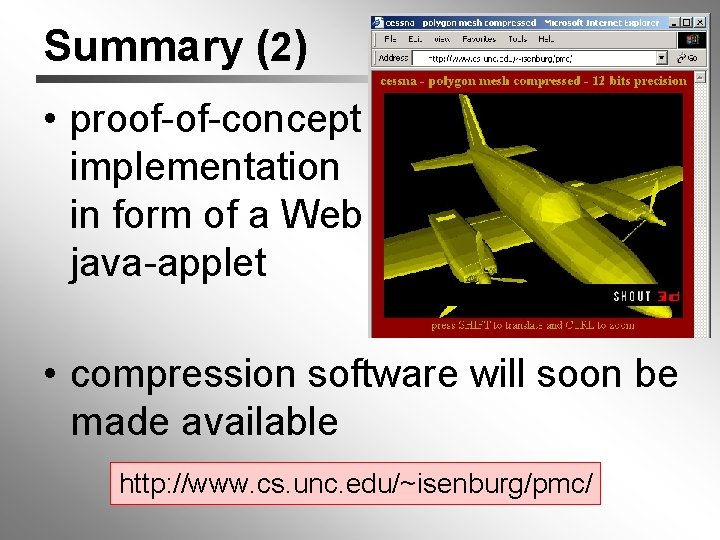
Summary (2) • proof-of-concept implementation in form of a Web java-applet • compression software will soon be made available http: //www. cs. unc. edu/~isenburg/pmc/

Future Work • a scientific way to find numbers for this “coefficient switching” • polygonification: – turn triangle meshes into polygon meshes for better compression

Acknowledgments funding: • ARC Télégéo grant of INRIA at Sophia-Antipolis logistics: • • Jack Snoeyink Olivier Devillers Agnès Clément Bessière Jean-Daniel Boissonnat

Thank You! http: //www. cs. unc. edu/~isenburg/pmc/