Compressible Flow CBE 150 A Transport Spring Semester

Compressible Flow CBE 150 A – Transport Spring Semester 2014

Goals • Describe how compressible flow differs from incompressible flow • Define criteria for situations in which compressible flow can be treated as incompressible • Provide example of situation in which compressibility cannot be neglected • Write basic equations for compressible flow • Describe a shape in which a compressible fluid can be accelerated to velocities above speed of sound (supersonic flow) CBE 150 A – Transport Spring Semester 2014

Basic Equations Five changeable quantities are important in compressible flow: 1. Cross-sectional area, S 2. Velocity, u 3. Pressure, p 4. Density, r 5. Temperature, T CBE 150 A – Transport Spring Semester 2014

Basic Equations Restrict focus to those systems in which properties are only changing in flow direction. Generally, cross-sectional area S is specified as a function of x. (S=S(x)) Need four equations to describe the other four variables. CBE 150 A – Transport Spring Semester 2014

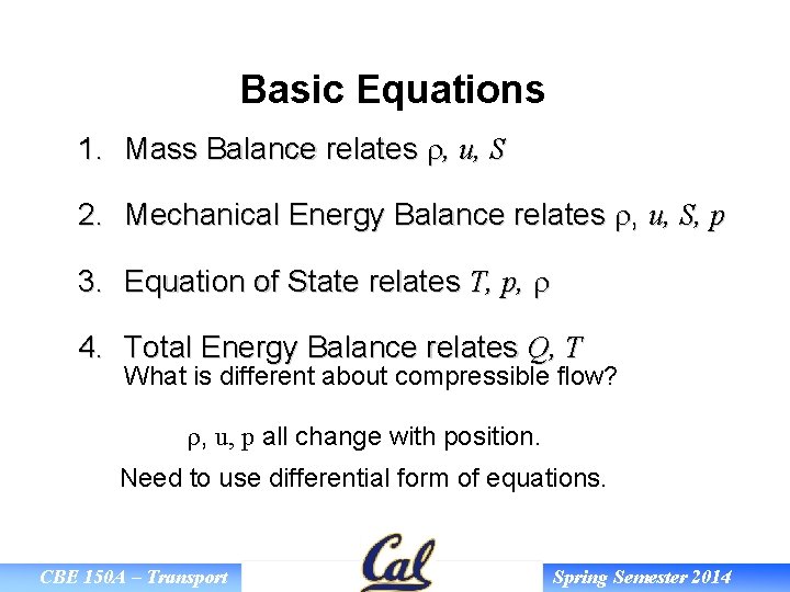
Basic Equations 1. Mass Balance relates r, u, S 2. Mechanical Energy Balance relates r, u, S, p 3. Equation of State relates T, p, r 4. Total Energy Balance relates Q, T What is different about compressible flow? r, u, p all change with position. Need to use differential form of equations. CBE 150 A – Transport Spring Semester 2014

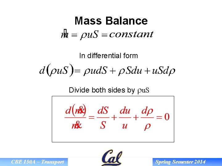
Mass Balance In differential form Divide both sides by ru. S CBE 150 A – Transport Spring Semester 2014

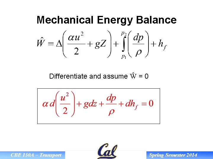
Mechanical Energy Balance Differentiate and assume Ŵ = 0 CBE 150 A – Transport Spring Semester 2014

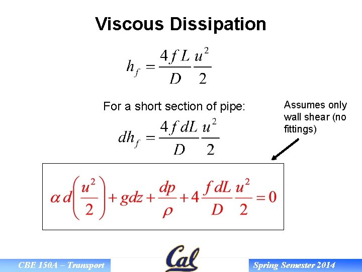
Viscous Dissipation For a short section of pipe: CBE 150 A – Transport Assumes only wall shear (no fittings) Spring Semester 2014

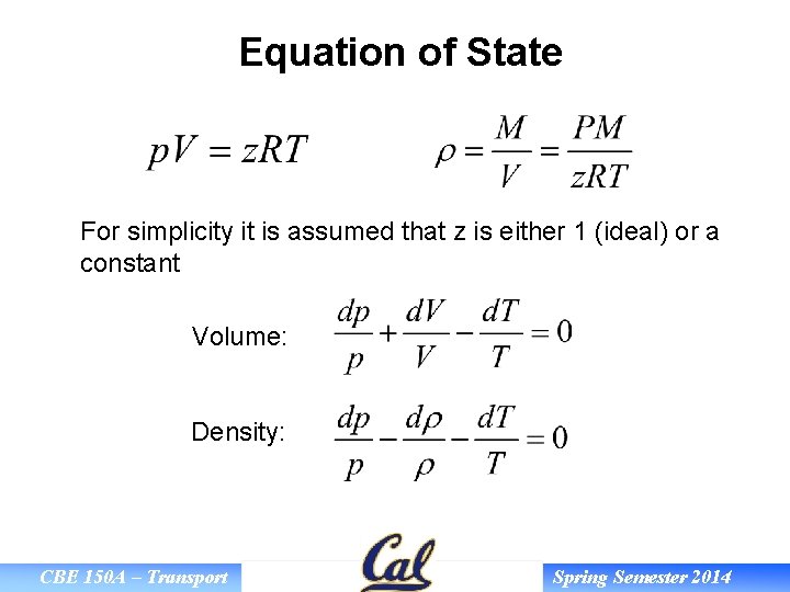
Equation of State For simplicity it is assumed that z is either 1 (ideal) or a constant Volume: Density: CBE 150 A – Transport Spring Semester 2014

Total Energy Balance For gases thermodynamics allows a better calculation of the heat transfer Q and changes in internal energy. These were terms that were previously included in the viscous dissipation term. The temperature of a flowing gas depends on: • Rate of heat transfer Q from environment. • Rate of viscous dissipation (significant in compressors). Included in work term Ŵc • Thermodynamic changes H. CBE 150 A – Transport Spring Semester 2014

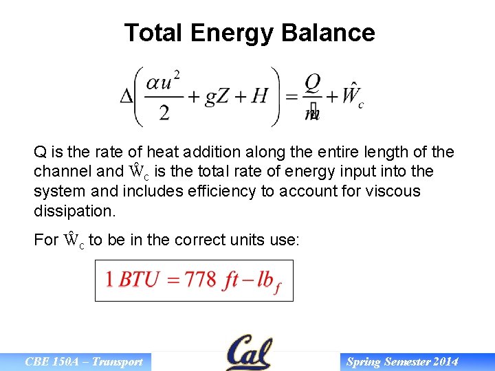
Total Energy Balance Q is the rate of heat addition along the entire length of the channel and Ŵc is the total rate of energy input into the system and includes efficiency to account for viscous dissipation. For Ŵc to be in the correct units use: CBE 150 A – Transport Spring Semester 2014

Compressible vs. Incompressible When can simpler incompressible equations be used? • Density change is not significant (<10%) • Fans, airflow through packed beds Mach number is a measure of the importance of density changes for compressible fluids. Rule of Thumb: NMa < 0. 3 assume incompressible CBE 150 A – Transport Spring Semester 2014

Isentropic Flow Adiabatic (Q = 0) and Reversible Isentropic (ΔS = 0) Venturi meter, Rocket propulsion CBE 150 A – Transport Spring Semester 2014

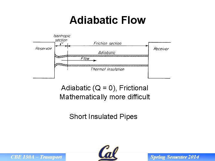
Adiabatic Flow Adiabatic (Q = 0), Frictional Mathematically more difficult Short Insulated Pipes CBE 150 A – Transport Spring Semester 2014

Isothermal Flow Isothermal, Frictional Long Uninsulated Pipes CBE 150 A – Transport Spring Semester 2014

Compressible Flow Through Pipes CBE 150 A – Transport Spring Semester 2014

Goals • Describe equations useful for analyzing isothermal, compressible flow through a constant diameter pipe. • Describe how Mach number and L are related for flow in a constant diameter pipe. • Use equations for isothermal flow to compute the flow rate of compressible fluids in constant diameter pipes. CBE 150 A – Transport Spring Semester 2014

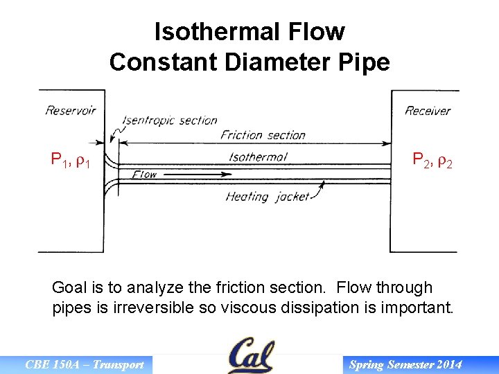
Isothermal Flow Constant Diameter Pipe P 1, r 1 P 2, r 2 Goal is to analyze the friction section. Flow through pipes is irreversible so viscous dissipation is important. CBE 150 A – Transport Spring Semester 2014

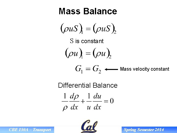
Mass Balance S is constant Mass velocity constant Differential Balance CBE 150 A – Transport Spring Semester 2014

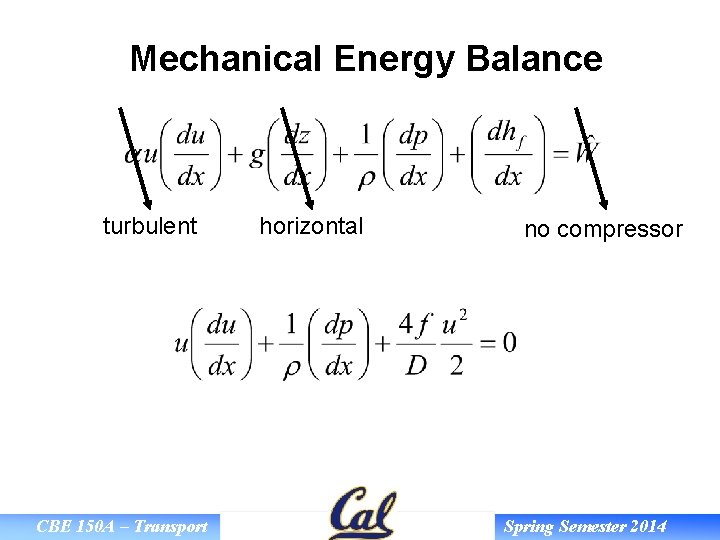
Mechanical Energy Balance turbulent CBE 150 A – Transport horizontal no compressor Spring Semester 2014

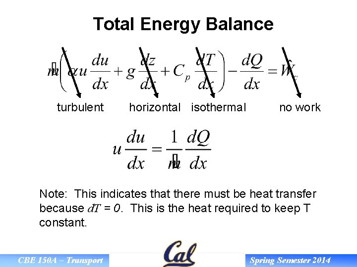
Total Energy Balance turbulent horizontal isothermal no work Note: This indicates that there must be heat transfer because d. T = 0. This is the heat required to keep T constant. CBE 150 A – Transport Spring Semester 2014

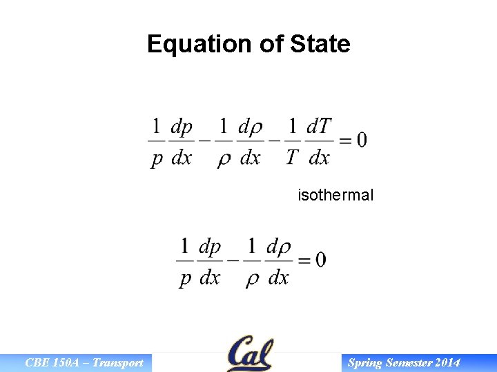
Equation of State isothermal CBE 150 A – Transport Spring Semester 2014

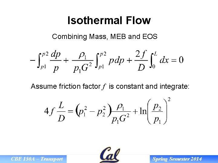
Isothermal Flow Combining Mass, MEB and EOS Assume friction factor f is constant and integrate: CBE 150 A – Transport Spring Semester 2014

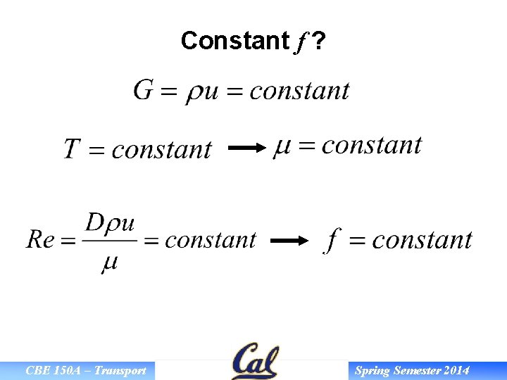
Constant f ? CBE 150 A – Transport Spring Semester 2014

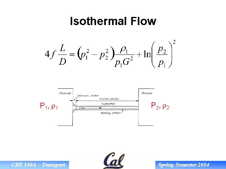
Isothermal Flow P 1, r 1 CBE 150 A – Transport P 2, r 2 Spring Semester 2014

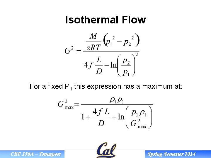
Isothermal Flow For a fixed P 1 this expression has a maximum at: CBE 150 A – Transport Spring Semester 2014

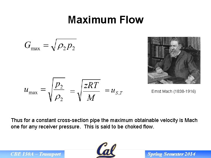
Maximum Flow Ernst Mach (1838 -1916) Thus for a constant cross-section pipe the maximum obtainable velocity is Mach one for any receiver pressure. This is said to be choked flow. CBE 150 A – Transport Spring Semester 2014

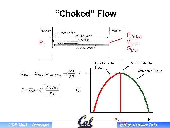
“Choked” Flow PCritical Vsonic GMax P 1 Unattainable Flows Sonic Velocity Attainable Flows G CBE 150 A – Transport PCritical P 1 Spring Semester 2014

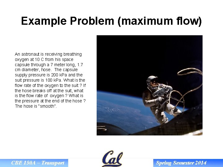
Example Problem (maximum flow) An astronaut is receiving breathing oxygen at 10 C from his space capsule through a 7 meter long, 1. 7 cm diameter, hose. The capsule supply pressure is 200 k. Pa and the suit pressure is 100 k. Pa. What is the flow rate of the oxygen to the suit ? If the hose breaks off at the suit, what is the flow rate of oxygen ? What is the pressure at the end of the hose ? The hose is “smooth”. CBE 150 A – Transport Spring Semester 2014

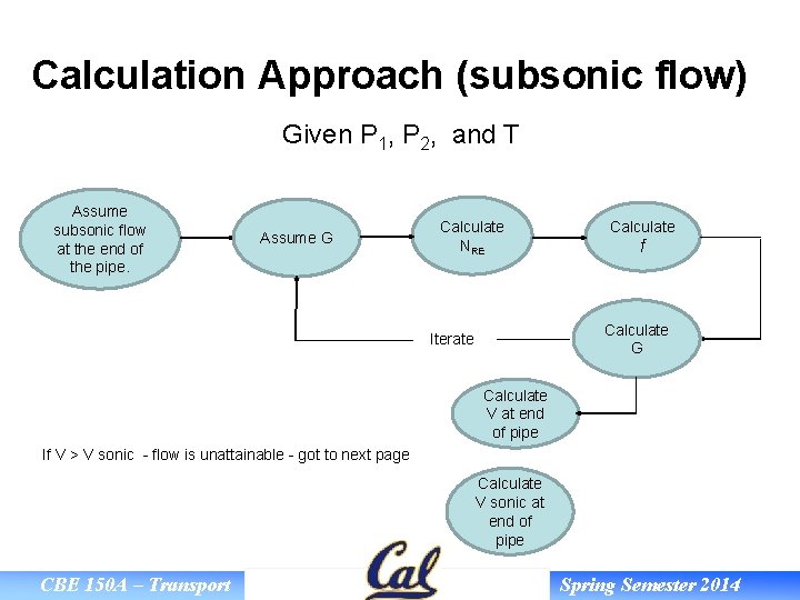
Calculation Approach (subsonic flow) Given P 1, P 2, and T Assume subsonic flow at the end of the pipe. Assume G Calculate NRE Calculate f Calculate G Iterate Calculate V at end of pipe If V > V sonic - flow is unattainable - got to next page Calculate V sonic at end of pipe CBE 150 A – Transport Spring Semester 2014

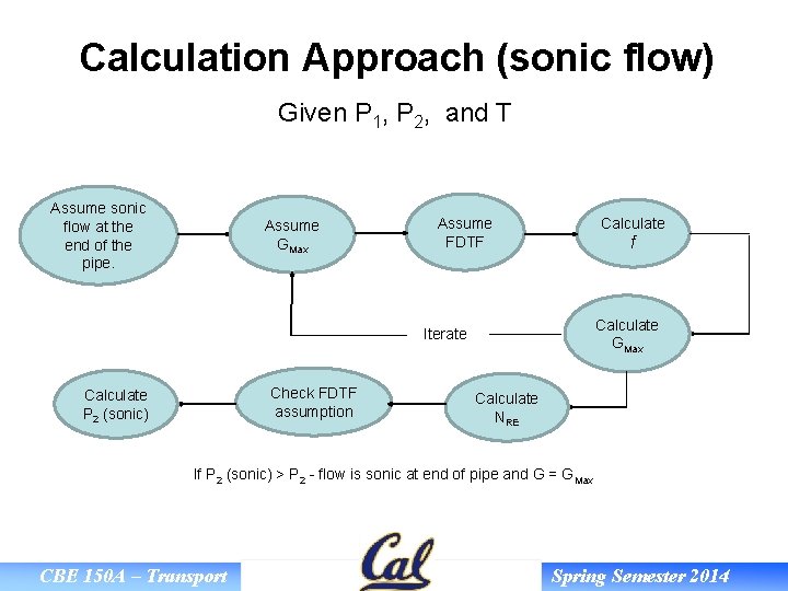
Calculation Approach (sonic flow) Given P 1, P 2, and T Assume sonic flow at the end of the pipe. Assume GMax Calculate Assume FDTF f Calculate GMax Iterate Check FDTF assumption Calculate P 2 (sonic) Calculate NRE If P 2 (sonic) > P 2 - flow is sonic at end of pipe and G = GMax CBE 150 A – Transport Spring Semester 2014

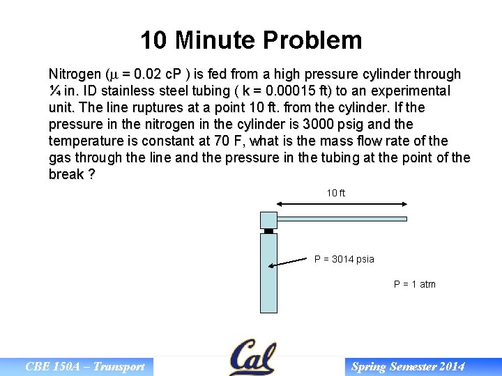
10 Minute Problem Nitrogen (m = 0. 02 c. P ) is fed from a high pressure cylinder through ¼ in. ID stainless steel tubing ( k = 0. 00015 ft) to an experimental unit. The line ruptures at a point 10 ft. from the cylinder. If the pressure in the nitrogen in the cylinder is 3000 psig and the temperature is constant at 70 F, what is the mass flow rate of the gas through the line and the pressure in the tubing at the point of the break ? 10 ft P = 3014 psia P = 1 atm CBE 150 A – Transport Spring Semester 2014

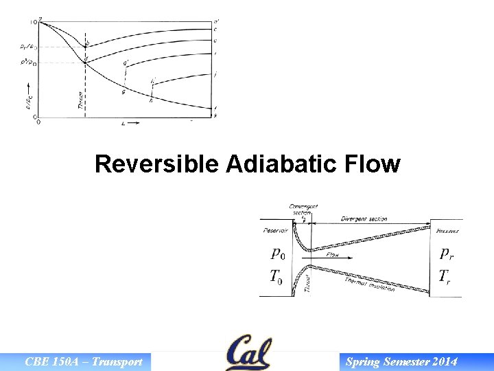
Reversible Adiabatic Flow CBE 150 A – Transport Spring Semester 2014

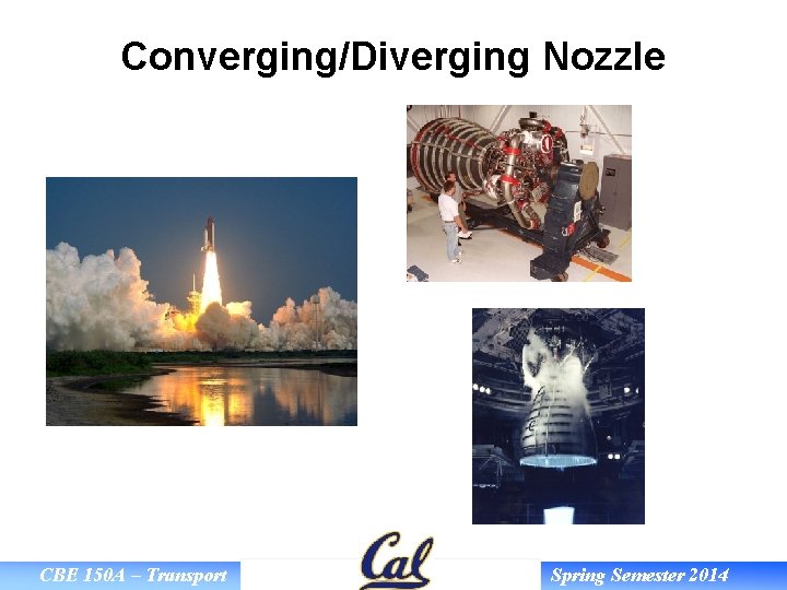
Converging/Diverging Nozzle CBE 150 A – Transport Spring Semester 2014

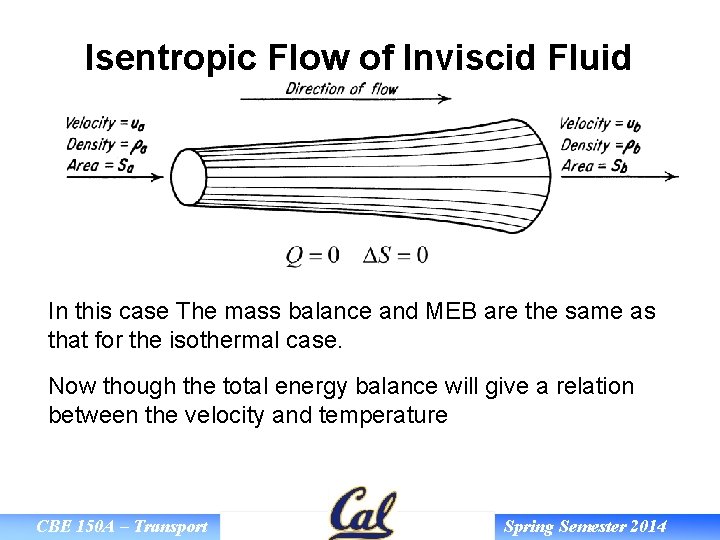
Isentropic Flow of Inviscid Fluid In this case The mass balance and MEB are the same as that for the isothermal case. Now though the total energy balance will give a relation between the velocity and temperature CBE 150 A – Transport Spring Semester 2014

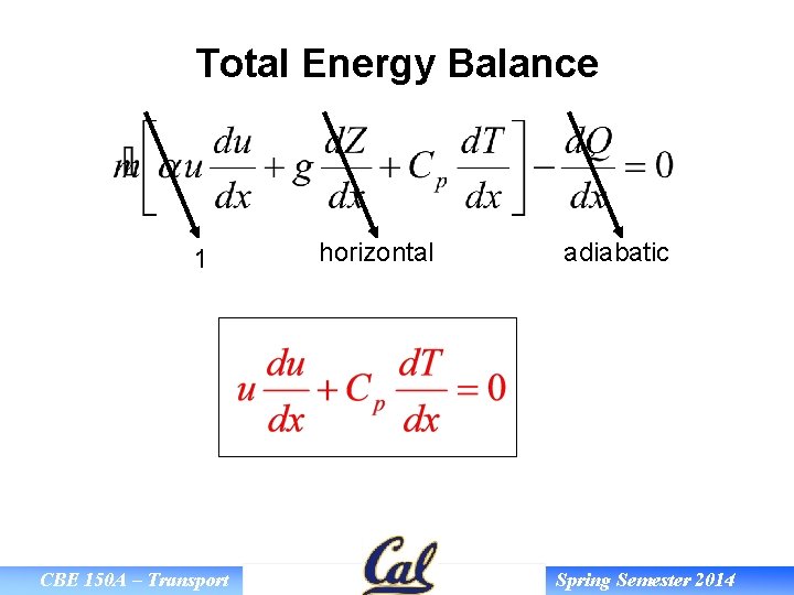
Total Energy Balance 1 CBE 150 A – Transport horizontal adiabatic Spring Semester 2014

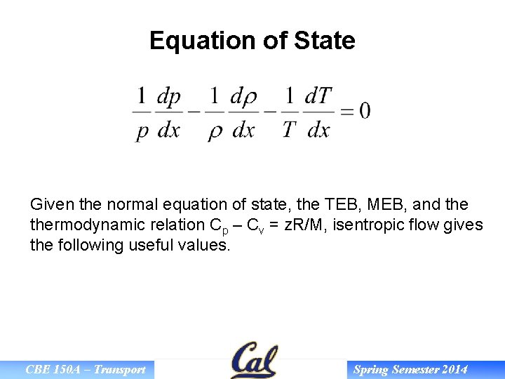
Equation of State Given the normal equation of state, the TEB, MEB, and thermodynamic relation Cp – Cv = z. R/M, isentropic flow gives the following useful values. CBE 150 A – Transport Spring Semester 2014

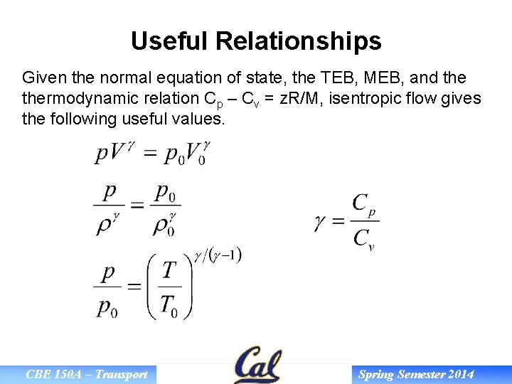
Useful Relationships Given the normal equation of state, the TEB, MEB, and thermodynamic relation Cp – Cv = z. R/M, isentropic flow gives the following useful values. CBE 150 A – Transport Spring Semester 2014

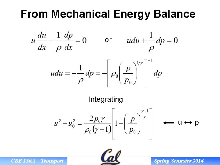
From Mechanical Energy Balance or Integrating u↔p CBE 150 A – Transport Spring Semester 2014

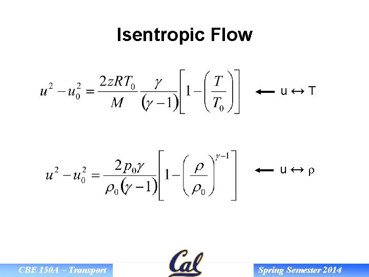
Isentropic Flow u↔T u↔r CBE 150 A – Transport Spring Semester 2014

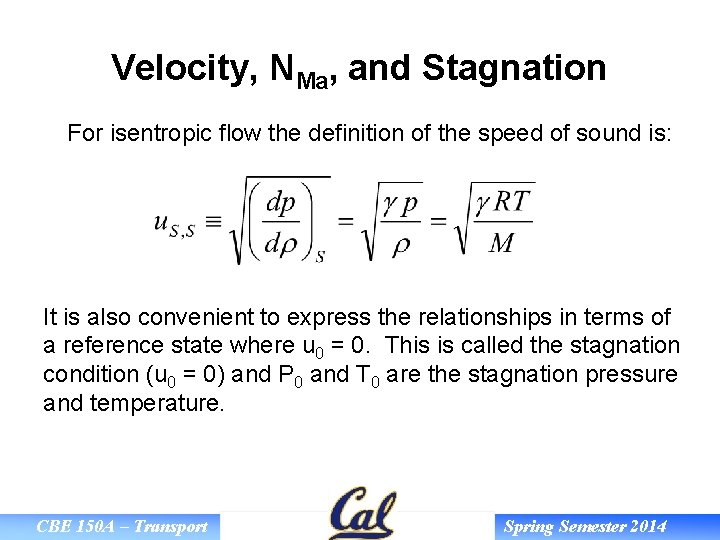
Velocity, NMa, and Stagnation For isentropic flow the definition of the speed of sound is: It is also convenient to express the relationships in terms of a reference state where u 0 = 0. This is called the stagnation condition (u 0 = 0) and P 0 and T 0 are the stagnation pressure and temperature. CBE 150 A – Transport Spring Semester 2014

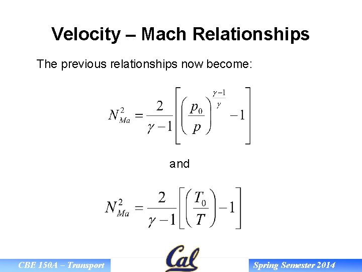
Velocity – Mach Relationships The previous relationships now become: and CBE 150 A – Transport Spring Semester 2014

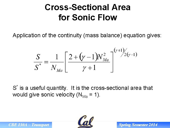
Cross-Sectional Area for Sonic Flow Application of the continuity (mass balance) equation gives: S* is a useful quantity. It is the cross-sectional area that would give sonic velocity (NMa = 1). CBE 150 A – Transport Spring Semester 2014

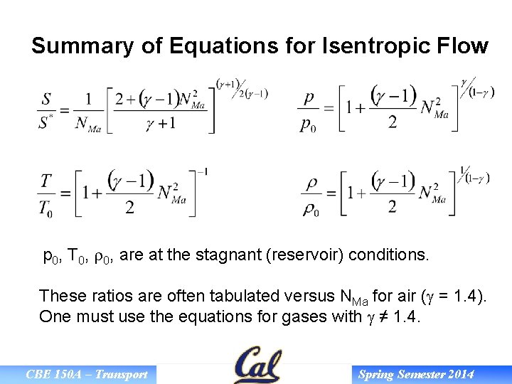
Summary of Equations for Isentropic Flow p 0, T 0, r 0, are at the stagnant (reservoir) conditions. These ratios are often tabulated versus NMa for air (g = 1. 4). One must use the equations for gases with g ≠ 1. 4. CBE 150 A – Transport Spring Semester 2014

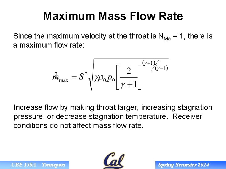
Maximum Mass Flow Rate Since the maximum velocity at the throat is NMa = 1, there is a maximum flow rate: Increase flow by making throat larger, increasing stagnation pressure, or decrease stagnation temperature. Receiver conditions do not affect mass flow rate. CBE 150 A – Transport Spring Semester 2014

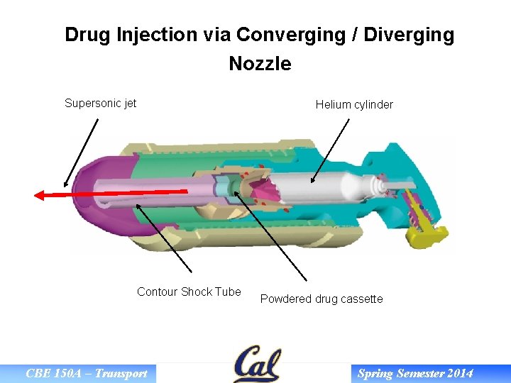
Drug Injection via Converging / Diverging Nozzle Supersonic jet Helium cylinder Contour Shock Tube CBE 150 A – Transport Powdered drug cassette Spring Semester 2014

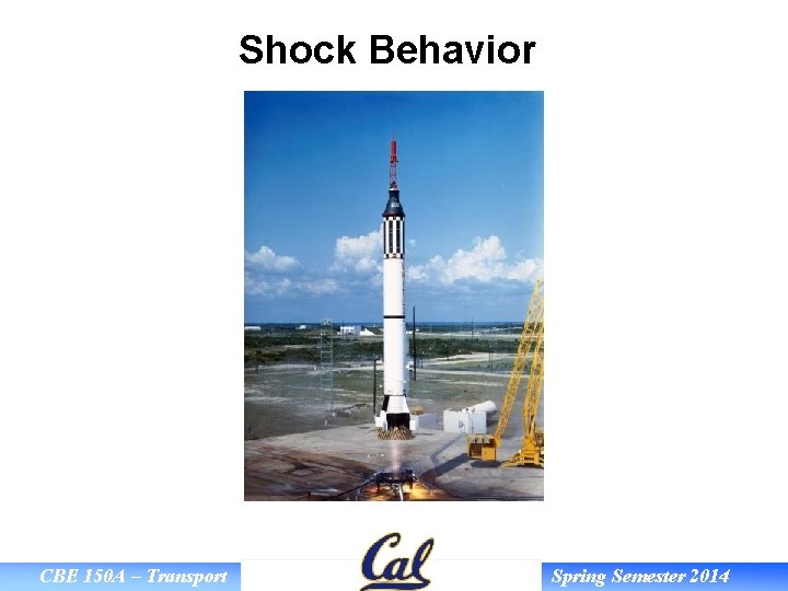
Shock Behavior CBE 150 A – Transport Spring Semester 2014

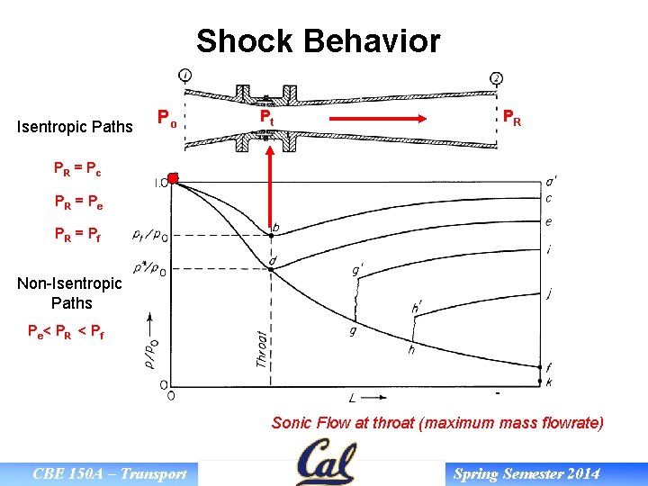
Shock Behavior Isentropic Paths Po Pt PR PR = P c PR = P e PR = P f Non-Isentropic Paths P e< P R < P f Sonic Flow at throat (maximum mass flowrate) CBE 150 A – Transport Spring Semester 2014

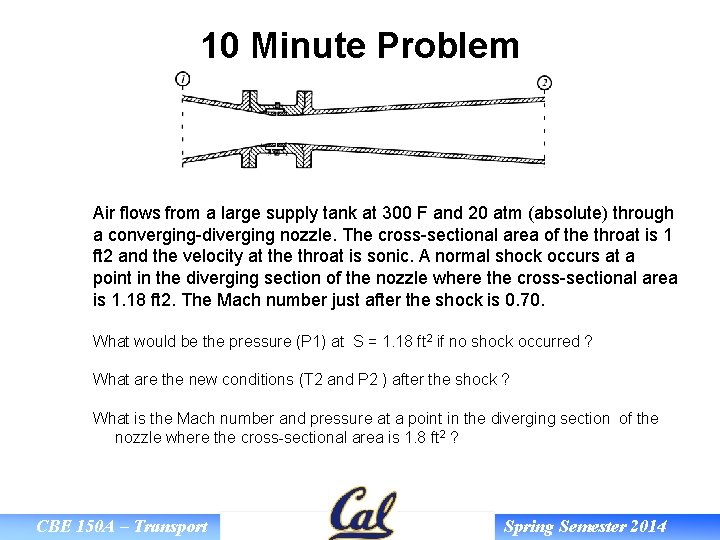
10 Minute Problem Air flows from a large supply tank at 300 F and 20 atm (absolute) through a converging-diverging nozzle. The cross-sectional area of the throat is 1 ft 2 and the velocity at the throat is sonic. A normal shock occurs at a point in the diverging section of the nozzle where the cross-sectional area is 1. 18 ft 2. The Mach number just after the shock is 0. 70. What would be the pressure (P 1) at S = 1. 18 ft 2 if no shock occurred ? What are the new conditions (T 2 and P 2 ) after the shock ? What is the Mach number and pressure at a point in the diverging section of the nozzle where the cross-sectional area is 1. 8 ft 2 ? CBE 150 A – Transport Spring Semester 2014

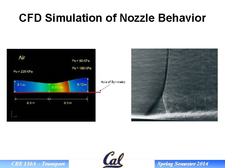
CFD Simulation of Nozzle Behavior CBE 150 A – Transport Spring Semester 2014