Compressed Sensing MRI 2016 12 15 Fully sampled

Compressed Sensing MRI 2016. 12. 15 Fully sampled 6 X undersampled with CS reconstruction

Lossy compression 失真壓縮 n n Reducing data size at cost of fidelity Widespread applied to music, images and movies: MP 3, JPEG, H. 264 (mpeg) Most useful data are highly compressible (link) Current model of data flow Acquisition Compression First lady of the Internet Application Lose 96% weight All bits of data are equal, but some bits are more equal than others.

Lossy compression 失真壓縮 At cost of fidelity? ? ? 14. 8 k. B Low resolution No compression Lossy compression 勝 “High” fidelity 2. 2 k. B High resolution with “less” fidelity

Compressibility and Sparsity Sparse: most numbers are zero or close to zero -128 x 0. 81 = 0 +127 = -0. 56 x x -0. 45 = = 0. 31 x x -0. 09 = = 0. 087 x x -0. 04 = = -0. 003 x x -0. 02 = = 0. 0001 x x 0. 007 = x 0. 0006 = =0 x x 0= = -0. 38 x = 0. 12 x = 0. 0002 x =0 x For example, under 2 D “discrete cosine transform” (JPEG 1992)

Compressibility and Sparsity Sparse: most numbers are zero or close to zero x 0. 81 = x -0. 45 = x -0. 09 = x -0. 04 = x -0. 02 = x 0. 007 = x 0. 0006 = -128 0 +127 = -0. 56 x = 0. 31 x = 0. 087 x = -0. 003 x = 0. 0001 x =0 x x 0= = -0. 38 x = 0. 12 x = 0. 0002 x =0 x Compression by discard small component of discrete cosine transform.

MR medical images are sparse Sparse after wavelet transform Sparse after finite difference transform Sparse after Fourier transform in time

Noncompressible image x 0. 62 = -128 0 +127 = -0. 48 x x -0. 60 = = 0. 46 x x -0. 59 = = 0. 40 x x -0. 56 = = -0. 35 x x -0. 56 = = 0. 32 x x 0. 54 = = 0. 32 x x 0. 52 = x 0. 52= = -0. 38 x = 0. 32 x = 0. 30 x = 0. 24 x White noise is not sparse to any transform, include DCT.

Compressed sensing (CS) n Current model of data flow Acquisition Compression Application First lady of the Internet n Lose 96% weight Compressed sensing data flow Compressed sensing Application Already compressed

Compressed sensing (CS) n n Current model gathers much more data than needed. Most could be discarded safely Acquisition device must be fast, cheap, plenty MR machine is slow, costly, scarce Exploit image sparsity, CS MRI is possible Compressed sensing Application Already compressed

A crash course of MRI principle k space Data acquisition image DFT

A crash course of MRI principle k space Data acquisition

A crash course of MRI principle k space Data acquisition

A crash course of MRI principle k space Data acquisition

A crash course of MRI principle k space Data acquisition

A crash course of MRI principle k space Data acquisition

A crash course of MRI principle k space Data acquisition

A crash course of MRI principle k space Data acquisition

A crash course of MRI principle k space Data acquisition image DFT

Full acquisition

Reconstruction with partial information Recovery? missing data DFT

Reconstruction with partial information Recovery? DFT a priori knowledge

Reconstruction with partial information Recovery? DFT DWT The a priori knowledge of compressed sensing is assuming the data is sparse in some basis, such as wavelet basis. sparse

It seems very difficult…. n n n Alice Bob Eve The a priori knowledge of compressed sensing is assuming the data is sparse in some basis, such as wavelet basis.

Localization make thing easier…. n n n 小王 (大喬 飾) 小柯 (小喬 飾) 小黃 (由各位飾演) The a priori knowledge of compressed sensing is assuming the data is sparse in some basis, such as wavelet basis.

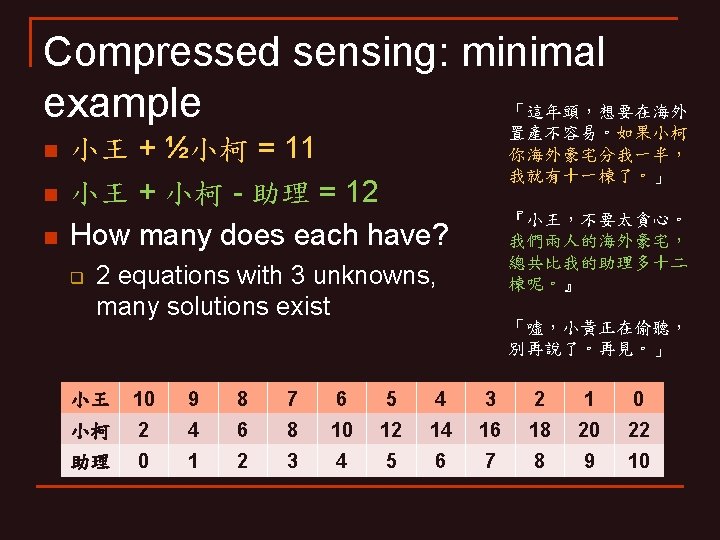
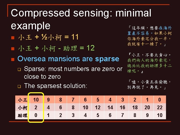
ℓ 0 , ℓ 1 and ℓ 2 (pseudo)norms n ℓ 0 pseudonorm: number of nonzero components q n ℓ 1 norm: sum of all components q n This is the definition of sparsity The sparsest solution is minimal in ℓ 1 “incidentally” ℓ 2 norm: root of sum-squares This solution is minimal in ℓ 0 and ℓ 1 (pseudo)norm, but not in ℓ 2 norm. 小王 10 9 8 7 6 5 4 3 2 1 0 小柯 2 4 6 8 10 12 14 16 18 20 22 助理 0 1 2 3 4 5 6 7 8 9 10

Incoherence n What if the scenario is: q q q n n 「小柯，我知道你的海外豪宅有兩棟。」 『但是我的助理一棟都沒有。』 We will never know how much does 小王 has Incoherence: Each sampled data should involves the basis as evenly as possible in the transformed domain Random sampling is incoherent relative to any basis, but not always applicable

如果各位要寫作業的話… n Sparsity: few nonzero components in the transformed domain n n Incoherence: Each sampled data should involves the basis as evenly as possible in the transformed domain Incoherence and sparsity are the keys to successful compressed sensing

How much sampling is enough? n n Signal size: n Sampling number: m Nyquist sampling For example, n = 512 x 512 = 262, 144, log n = 5. 4

How much sampling is enough? n n n Signal size: n Sampling number: m Sparse: S nonzero component Nyquist sampling “Just enough” sampling For example, n = 512 x 512 = 262, 144, log n = 5. 4

How much sampling is enough? n n Signal size: n Sampling number: m Sparse: S nonzero component Incoherence: u q u = 1 maximally incoherent, usually u ~ 2 Nyquist sampling Compressed sensing “Just enough” sampling For example, n = 512 x 512 = 262, 144, log n = 5. 4

Compressed sensing, theorem 1 n Randomly acquiring m samples, m > a (strictly) S-sparse signal is recovered with probability > 1 - Find k in Rn Minimize || DWT(DFT(k)) ||1 Subject to ki = Ki i = 1… m Convex optimization problem Efficient algorithm exists

Compressed sensing, theorem 1 DFT DWT sparse Find k in Rn Minimize || DWT(DFT(k)) ||1 Subject to ki = Ki i = 1… m Convex optimization problem Efficient algorithm exists

Compressed sensing, theorem 1 n Randomly acquiring m samples, m > a (strictly) S-sparse signal is recovered with probability > 1 - What if the signal is only approximately S-sparse, and noisy?

Compressed sensing, theorem 2 approx. S-sparse recovery error noisy level Find k in Rn Minimize || DWT(DFT(k)) ||1 Subject to ki ≒ Ki i = 1… m Convex optimization problem Efficient algorithm

Point spread function (PSF) in 1 dimension: Thresholding random sampling Regular sampling Imaging space k-space Ambiguity! 模擬 subsampling 所產生的雜訊 “模擬 subsampling 所產生的雜訊”: Point spread function The more evenly spread out of the noise, the better.

Point spread function in 2 -dimension “模擬 subsampling 所產生的雜訊”: Point spread function The more evenly spread out of the noise, the better: incoherence

Incoherent sampling: PSF in 2 dimension “模擬 subsampling 所產生的雜訊”: Point spread function The more evenly spread out of the noise, the better: incoherence

Summary of compressed sensing MRI n n MRI images are sparse Nonrandom incoherent k-space trajectories Compressed sensing can achieve similar images quality using sub-Nyquist sampling 5 X to 10 X speed up q Advantages…

Summary of compressed sensing MRI n n MRI images are sparse Nonrandom incoherent k-space trajectories Compressed sensing can achieve similar images quality using sub-Nyquist sampling Make 5 X to 10 X speed up Ultrafast screening for stroke More NEX Larger FOV timeconsuming One breath-hold scan probable No motion body images artifact No anesthesia for babies No more Higher overtime work resolution

What’s next? Beyond sparsity n n n Sparsity is a rudimentary a priori knowledge Can we expand a priori knowledge by machine learning? Beyond sparsity

Thanks for your attention

It’s Showtime! Original image 6 X subsampling with CS Original 6 X subsampling

It’s Showtime! Original image 6 X subsampling with CS Original 6 X subsampling

It’s Showtime! Free breathing whole liver perfusion One breath-hold whole heart perfusion

It’s Showtime! Submillimeter resolution T 1 WI +C in a 8 -year-old boy Radiology. 2010 August; 256(2): 607– 616

It’s Showtime! Breath-hold CE MRA Radiology. 2010 August; 256(2): 607– 616

It’s Showtime! 3 -year-old boy with left hepatic lobe transplant, SSFP MRCP Radiology. 2010 August; 256(2): 607– 616

Thanks for your attention

Nyquist rate: comprehensive sampling n n n Sampling freq > maximal freq in signal * 2 Guarantee perfect signal reconstruction Sub-Nyquist sampling q q Aliasing 高頻訊號誤為低頻訊號 Moiré pattern; wagon-wheel effect; phase wrapping.

Compressed sensing MRI (finally!) Limitation in maximal slew rate and gradient field

Compressed sensing MRI The k-space is traversed by various trajectory, and sampled with Nyquist rate. The coverage determines resolution; the density determines FOV. Violation of the sampling requirement results in imaging artifacts.

Compressed sensing MRI High quality image Loss of resolution Small FOV wrapping Random noise

To really achieve incoherence in MRI n n Random sampling is incoherent to any transform In MRI, real random sampling is not practical q q n Slewmax and Gmax K-space trajectory should be smooth lines Devise nonrandom incoherent sampling with smooth k-space trajectories

Incoherent sampling in time Exploit sparsity after Fourier transform in time

An easier(? ) diagram non-zero component sampling number “Just enough” sampling number signal size probability of accurate reconstruction Fully sampled at Nyquist rate

An easier(? ) diagram non-zero component sampling number “Just enough” sampling number signal size probability of accurate reconstruction Fully sampled at Nyquist rate This is a hyperbola. Sparsity ratio S/n = 0. 2

A more elaborate example –sub-Nyquist sampling Random sampling is maximally incoherent “random” noise Fourier transform Imaging space k-space Sampling in regular interval is not incoherent to Fourier basis Ambiguity! Aliasing

A more elaborate example –sub-Nyquist sampling thresholding Ambiguity! 無路可走 模擬subsampling 所產生的雜訊