Compressed Sensing in Multimedia CodingProcessing Trac D Tran

Compressed Sensing in Multimedia Coding/Processing Trac D. Tran ECE Department The Johns Hopkins University Baltimore, MD 21218

Outline u Compressed Sensing: Quick Overview § Motivations. Toy Examples § Incoherent Bases and Restrictive Isometry Property § Decoding Strategy § L 0 versus L 1 versus L 2 § Basis Pursuit and Matching Pursuit u Compressed Sensing in Image/Video Processing § § 2 D Separable Measurement Ensemble (SME) Face Recognition Distributed compressed video sensing (DISCOS) Layered compressed sensing for robust video transmission

Compressed Sensing History u u Emmanuel Candès and Terence Tao, ”Decoding by linear programming” IEEE Trans. on Information Theory, 51(12), pp. 4203 - 4215, December 2005 Emmanuel Candès, Justin Romberg, and Terence Tao, ”Robust uncertainty principles: Exact signal reconstruction from highly incomplete frequency information, ” IEEE Trans. on Information Theory, 52(2) pp. 489 - 509, Feb. 2006. David Donoho, ”Compressed sensing, ” IEEE Trans. on Information Theory, 52(4), pp. 1289 - 1306, Apr. 2006. Emmanuel Candès and Michael Wakin, ”An introduction to compressive sampling, ” IEEE Signal Processing Magazine, 25(2), pp. 21 - 30, Mar. 2008.

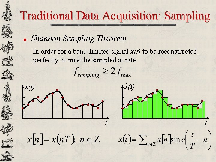
Traditional Data Acquisition: Sampling u Shannon Sampling Theorem In order for a band-limited signal x(t) to be reconstructed perfectly, it must be sampled at rate ^ x(t) t t

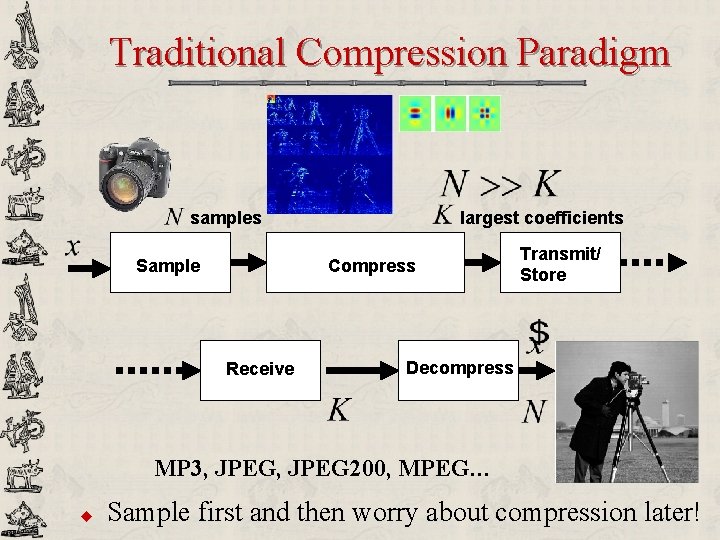
Traditional Compression Paradigm samples Sample largest coefficients Compress Receive Transmit/ Store Decompress MP 3, JPEG 200, MPEG… u Sample first and then worry about compression later!

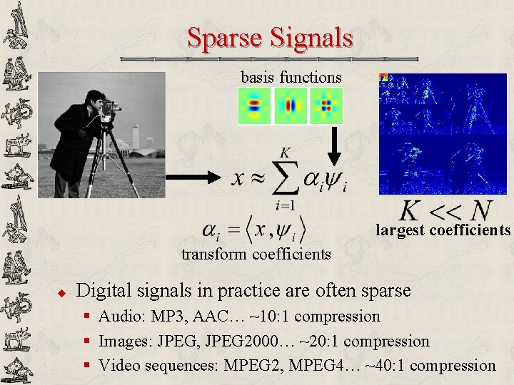
Sparse Signals basis functions largest coefficients transform coefficients u Digital signals in practice are often sparse § Audio: MP 3, AAC… ~10: 1 compression § Images: JPEG, JPEG 2000… ~20: 1 compression § Video sequences: MPEG 2, MPEG 4… ~40: 1 compression

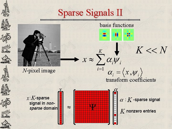
Sparse Signals II basis functions N-pixel image transform coefficients : -sparse signal in nonsparse domain : -sparse signal nonzero entries

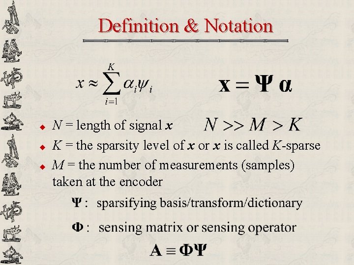
Definition & Notation u u u N = length of signal x K = the sparsity level of x or x is called K-sparse M = the number of measurements (samples) taken at the encoder

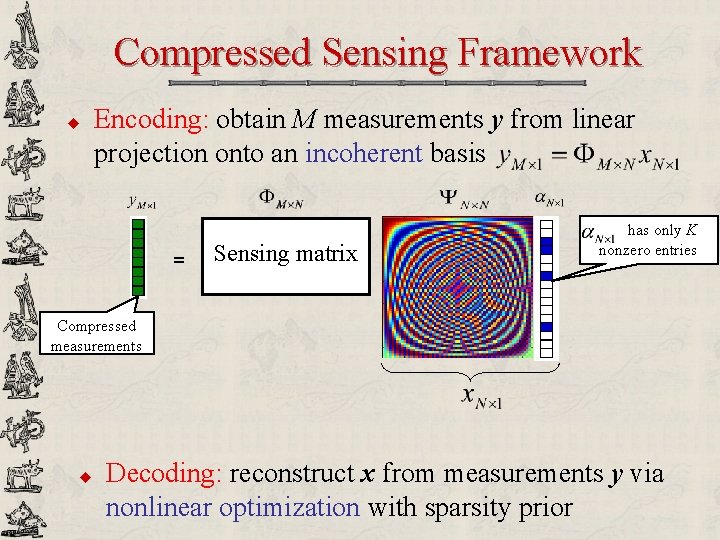
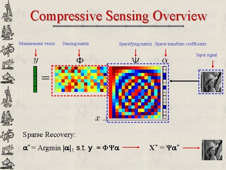
Compressed Sensing Framework u Encoding: obtain M measurements y from linear projection onto an incoherent basis = Sensing matrix has only K nonzero entries Compressed measurements u Decoding: reconstruct x from measurements y via nonlinear optimization with sparsity prior

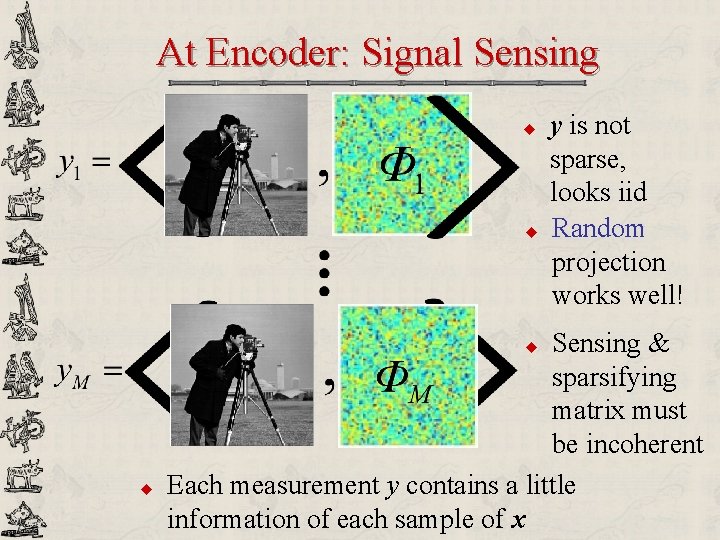
At Encoder: Signal Sensing u u Sensing & sparsifying matrix must be incoherent Each measurement y contains a little information of each sample of x u u y is not sparse, looks iid Random projection works well!

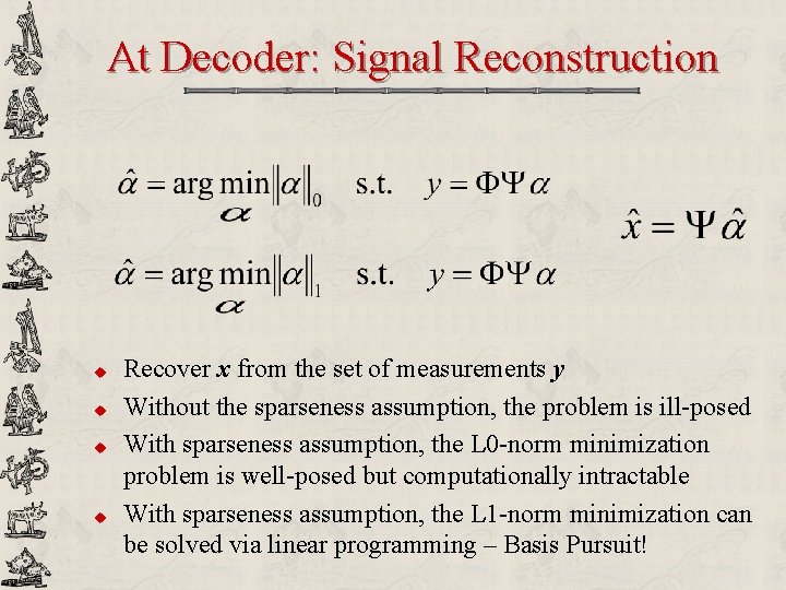
At Decoder: Signal Reconstruction u u Recover x from the set of measurements y Without the sparseness assumption, the problem is ill-posed With sparseness assumption, the L 0 -norm minimization problem is well-posed but computationally intractable With sparseness assumption, the L 1 -norm minimization can be solved via linear programming – Basis Pursuit!

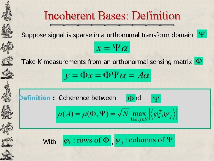
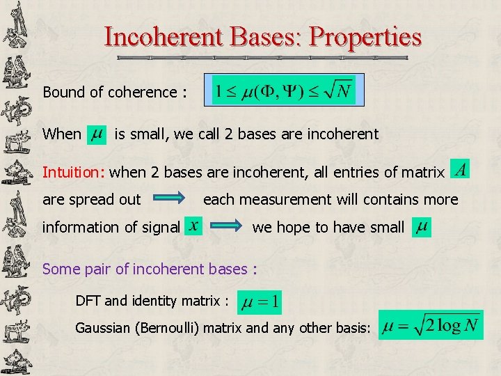
Incoherent Bases: Definition Suppose signal is sparse in a orthonomal transform domain Take K measurements from an orthonormal sensing matrix Definition : Coherence between and T With ,

Incoherent Bases: Properties Bound of coherence : When is small, we call 2 bases are incoherent Intuition: when 2 bases are incoherent, all entries of matrix are spread out each measurement will contains more information of signal we hope to have small Some pair of incoherent bases : DFT and identity matrix : Gaussian (Bernoulli) matrix and any other basis:

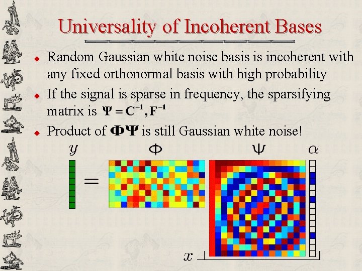
Universality of Incoherent Bases u u u Random Gaussian white noise basis is incoherent with any fixed orthonormal basis with high probability If the signal is sparse in frequency, the sparsifying matrix is Product of is still Gaussian white noise!

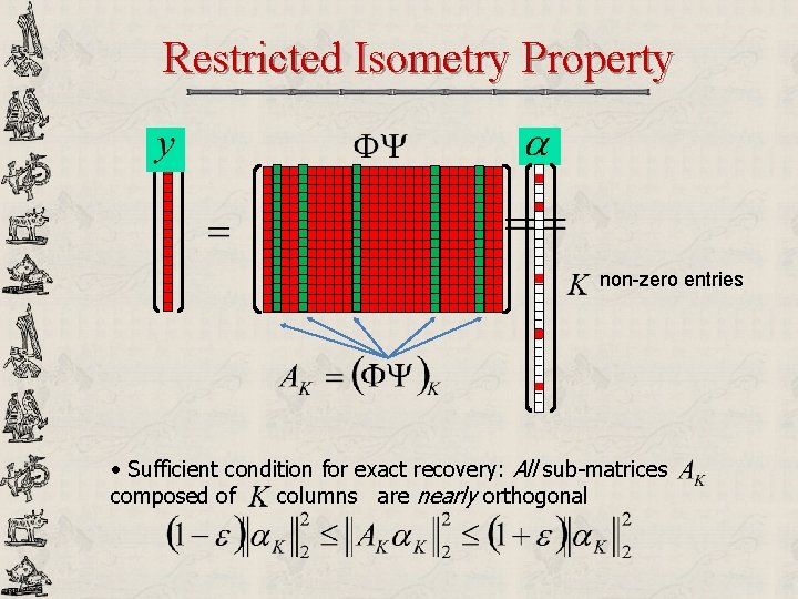
Restricted Isometry Property non-zero entries • Sufficient condition for exact recovery: All sub-matrices composed of columns are nearly orthogonal

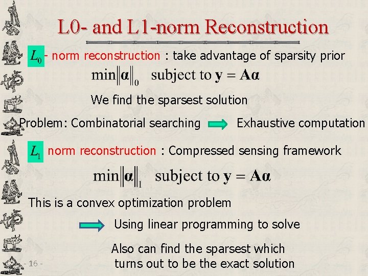
L 0 - and L 1 -norm Reconstruction - norm reconstruction : take advantage of sparsity prior We find the sparsest solution Problem: Combinatorial searching Exhaustive computation - norm reconstruction : Compressed sensing framework This is a convex optimization problem Using linear programming to solve - 16 - Also can find the sparsest which turns out to be the exact solution

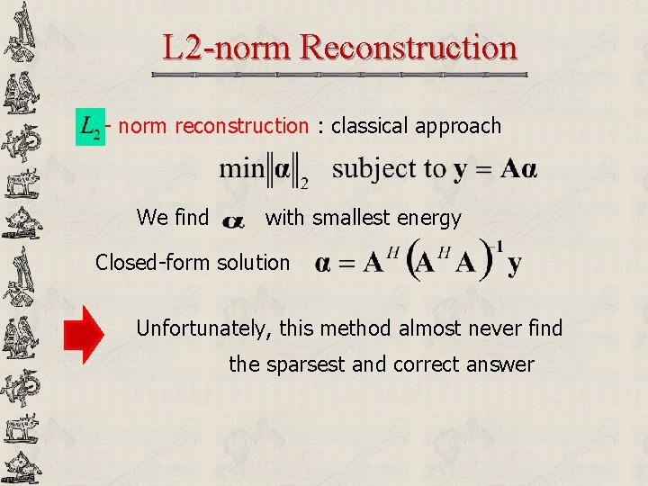
L 2 -norm Reconstruction - norm reconstruction : classical approach We find with smallest energy Closed-form solution Unfortunately, this method almost never find the sparsest and correct answer

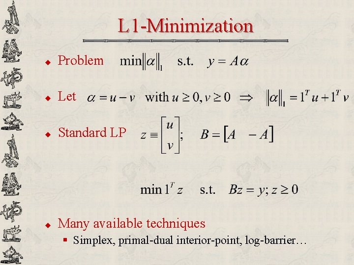
L 1 -Minimization u Problem u Let u Standard LP u Many available techniques § Simplex, primal-dual interior-point, log-barrier…

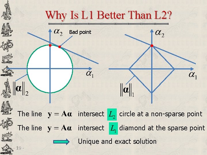
Why Is L 1 Better Than L 2? Bad point The line intersect circle at a non-sparse point The line intersect diamond at the sparse point - 19 - Unique and exact solution

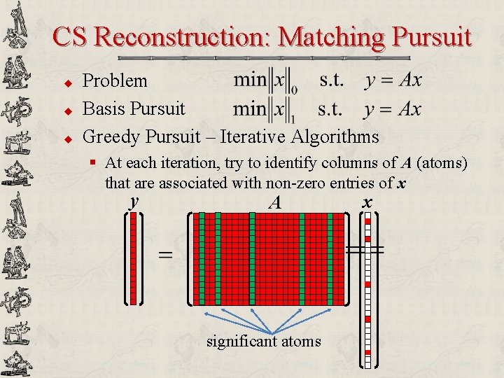
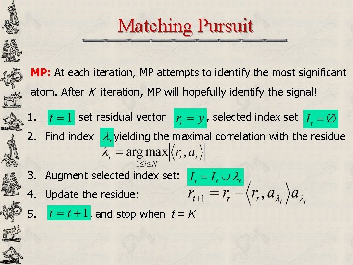
CS Reconstruction: Matching Pursuit u u u Problem Basis Pursuit Greedy Pursuit – Iterative Algorithms § At each iteration, try to identify columns of A (atoms) that are associated with non-zero entries of x y A significant atoms x

Matching Pursuit MP: At each iteration, MP attempts to identify the most significant atom. After K iteration, MP will hopefully identify the signal! 1. , set residual vector 2. Find index yielding the maximal correlation with the residue 3. Augment selected index set: 4. Update the residue: 5. , selected index set , and stop when t = K

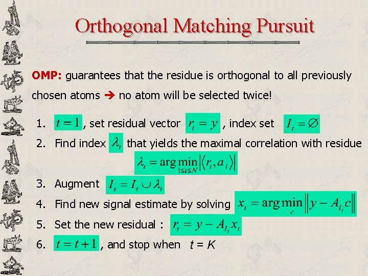
Orthogonal Matching Pursuit OMP: guarantees that the residue is orthogonal to all previously chosen atoms no atom will be selected twice! 1. , set residual vector 2. Find index , index set that yields the maximal correlation with residue 3. Augment 4. Find new signal estimate by solving 5. Set the new residual : 6. , and stop when t = K

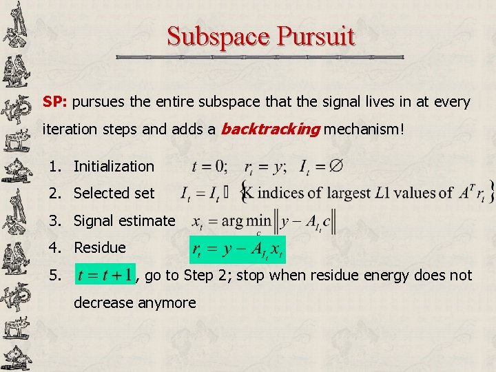
Subspace Pursuit SP: pursues the entire subspace that the signal lives in at every iteration steps and adds a backtracking mechanism! 1. Initialization 2. Selected set 3. Signal estimate 4. Residue 5. , go to Step 2; stop when residue energy does not decrease anymore

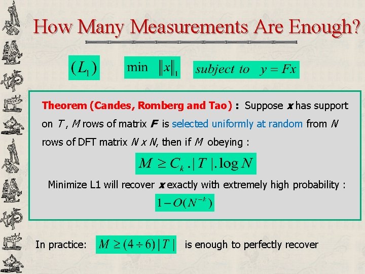
How Many Measurements Are Enough? Theorem (Candes, Romberg and Tao) : Suppose x has support on T , M rows of matrix F is selected uniformly at random from N rows of DFT matrix N x N, then if M obeying : Minimize L 1 will recover x exactly with extremely high probability : In practice: is enough to perfectly recover

CS in Multimedia Coding/Processing u Practical Compressed Sensing or Sparse Signal Processing § § § § § One-pixel camera 2 D separable measurement ensemble for image/video Face recognition Speech recognition Distributed compressed video sensing Layered compressed-sensing robust video transmission Video denoising Video super-resolution Multiple description coding MRI application

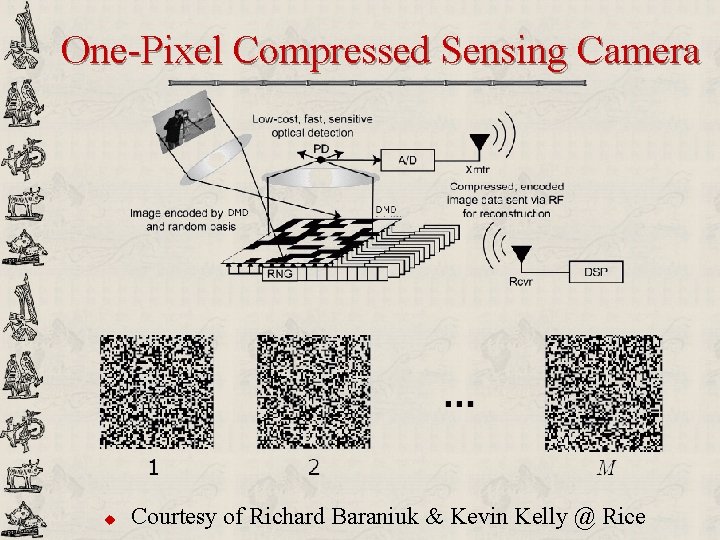
One-Pixel Compressed Sensing Camera u Courtesy of Richard Baraniuk & Kevin Kelly @ Rice

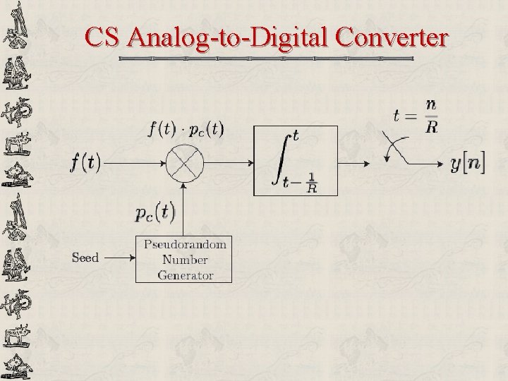
CS Analog-to-Digital Converter

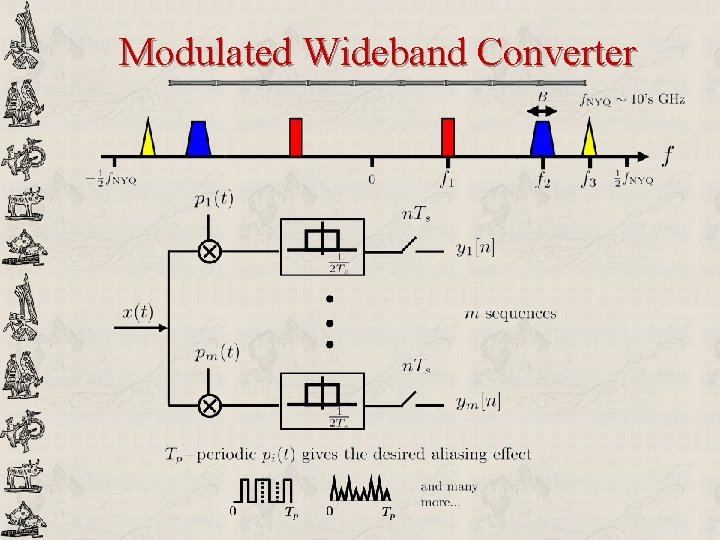
Modulated Wideband Converter

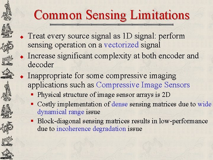
Common Sensing Limitations u u u Treat every source signal as 1 D signal: perform sensing operation on a vectorized signal Increase significant complexity at both encoder and decoder Inappropriate for some compressive imaging applications such as Compressive Image Sensors § Physical structure of image sensor arrays is 2 D § Costly implementation of dense sensing matrices due to wide dynamical range issue § Block-diagonal sensing matrices results in low-performance due to incoherence degradation issue

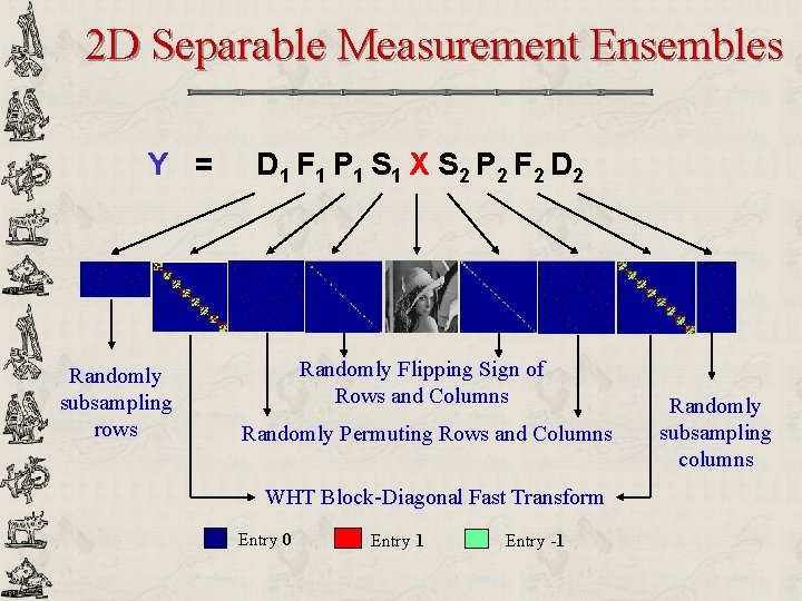
2 D Separable Measurement Ensembles Y = Randomly subsampling rows D 1 F 1 P 1 S 1 X S 2 P 2 F 2 D 2 Randomly Flipping Sign of Rows and Columns Randomly Permuting Rows and Columns WHT Block-Diagonal Fast Transform Entry 0 Entry 1 Entry -1 Randomly subsampling columns

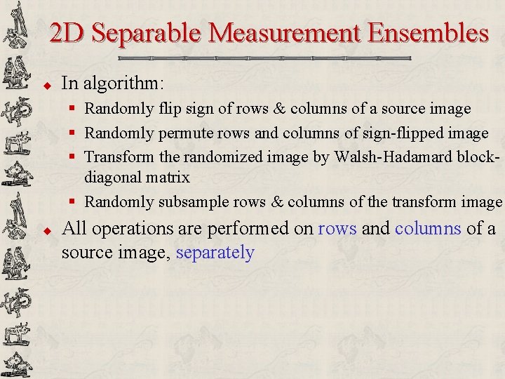
2 D Separable Measurement Ensembles u In algorithm: § Randomly flip sign of rows & columns of a source image § Randomly permute rows and columns of sign-flipped image § Transform the randomized image by Walsh-Hadamard blockdiagonal matrix § Randomly subsample rows & columns of the transform image u All operations are performed on rows and columns of a source image, separately

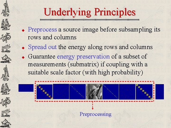
Underlying Principles u u u Preprocess a source image before subsampling its rows and columns Spread out the energy along rows and columns Guarantee energy preservation of a subset of measurements (submatrix) if coupling with a suitable scale factor (with high probability) Preprocessing

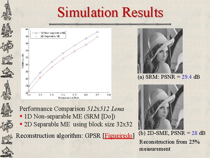
Simulation Results (a) SRM: PSNR = 29. 4 d. B Performance Comparison 512 x 512 Lena § 1 D Non-separable ME (SRM [Do]) § 2 D Separable ME using block size 32 x 32 Reconstruction algorithm: GPSR [Figueiredo] (b) 2 D-SME, PSNR = 28 d. B Reconstruction from 25% measurement

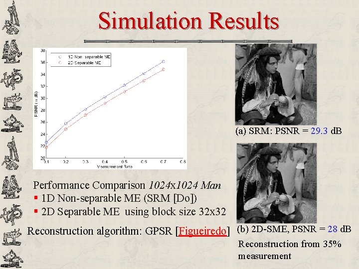
Simulation Results (a) SRM: PSNR = 29. 3 d. B Performance Comparison 1024 x 1024 Man § 1 D Non-separable ME (SRM [Do]) § 2 D Separable ME using block size 32 x 32 Reconstruction algorithm: GPSR [Figueiredo] (b) 2 D-SME, PSNR = 28 d. B Reconstruction from 35% measurement

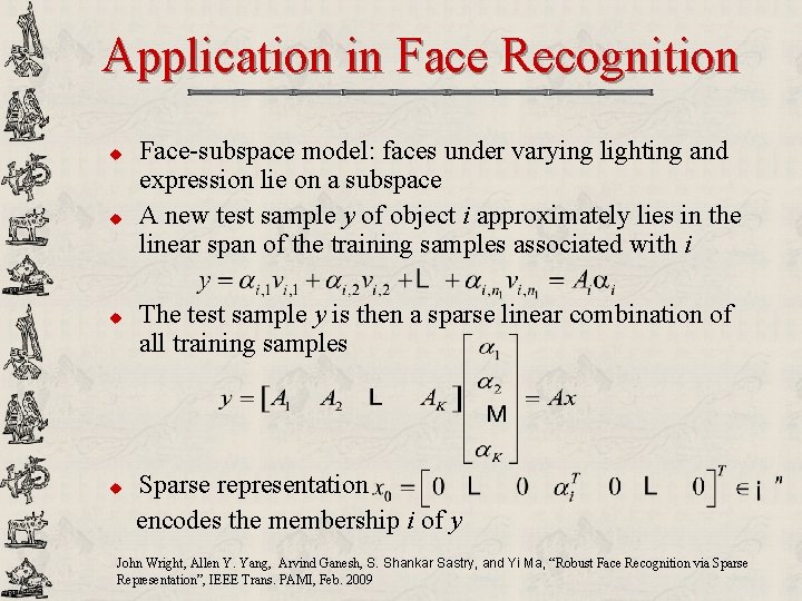
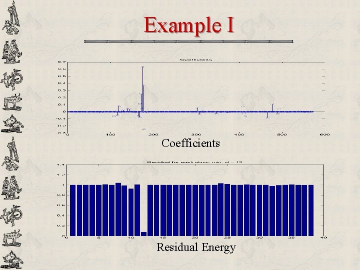
Application in Face Recognition u u Face-subspace model: faces under varying lighting and expression lie on a subspace A new test sample y of object i approximately lies in the linear span of the training samples associated with i The test sample y is then a sparse linear combination of all training samples Sparse representation encodes the membership i of y John Wright, Allen Y. Yang, Arvind Ganesh, S. Shankar Sastry, and Yi Ma, “Robust Face Recognition via Sparse Representation”, IEEE Trans. PAMI, Feb. 2009

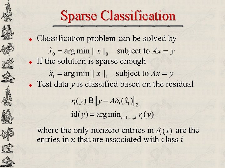
Sparse Classification u Classification problem can be solved by u If the solution is sparse enough u Test data y is classified based on the residual where the only nonzero entries in are the entries in x that are associated with class i

Example I Coefficients Residual Energy

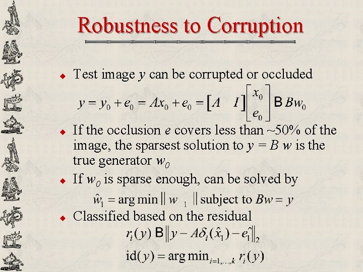
Robustness to Corruption u u Test image y can be corrupted or occluded If the occlusion e covers less than ~50% of the image, the sparsest solution to y = B w is the true generator w 0 If w 0 is sparse enough, can be solved by Classified based on the residual

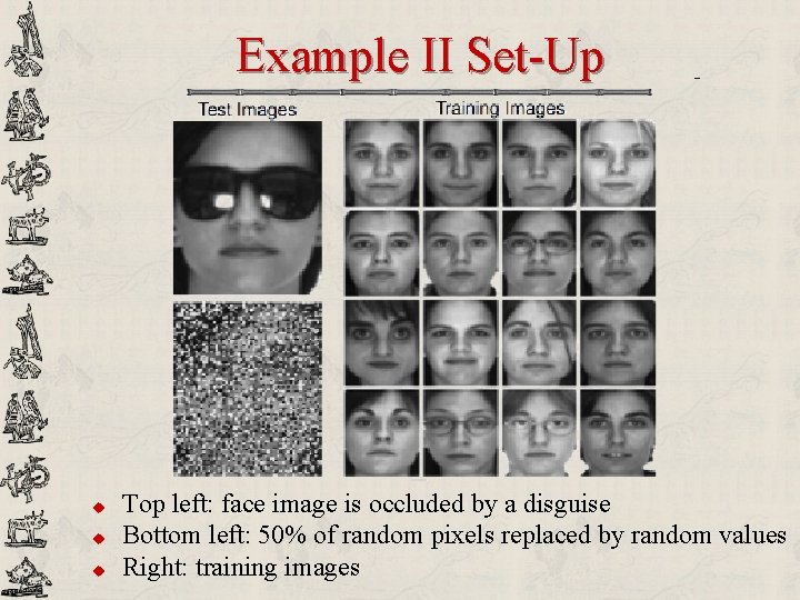
Example II Set-Up u u u Top left: face image is occluded by a disguise Bottom left: 50% of random pixels replaced by random values Right: training images

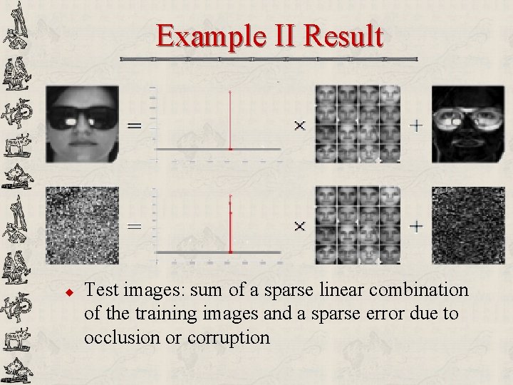
Example II Result u Test images: sum of a sparse linear combination of the training images and a sparse error due to occlusion or corruption

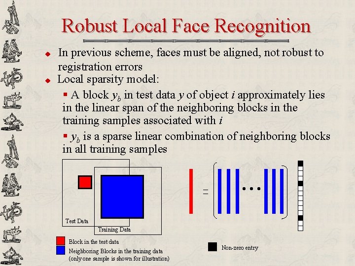
Robust Local Face Recognition u u In previous scheme, faces must be aligned, not robust to registration errors Local sparsity model: § A block yb in test data y of object i approximately lies in the linear span of the neighboring blocks in the training samples associated with i § yb is a sparse linear combination of neighboring blocks in all training samples • • • Test Data Training Data Block in the test data Neighboring Blocks in the training data (only one sample is shown for illustration) Non-zero entry

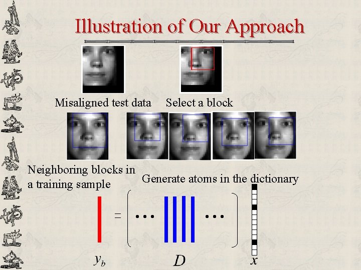
Illustration of Our Approach Misaligned test data Select a block Neighboring blocks in Generate atoms in the dictionary a training sample • • •

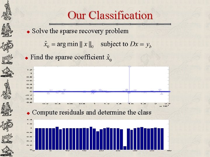
Our Classification u u u Solve the sparse recovery problem Find the sparse coefficient Compute residuals and determine the class

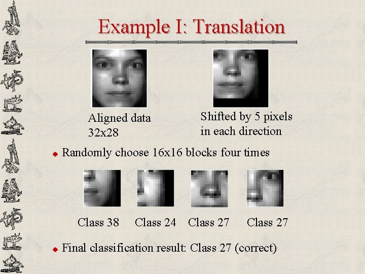
Example I: Translation Aligned data 32 x 28 u Randomly choose 16 x 16 blocks four times Class 38 u Shifted by 5 pixels in each direction Class 24 Class 27 Final classification result: Class 27 (correct)

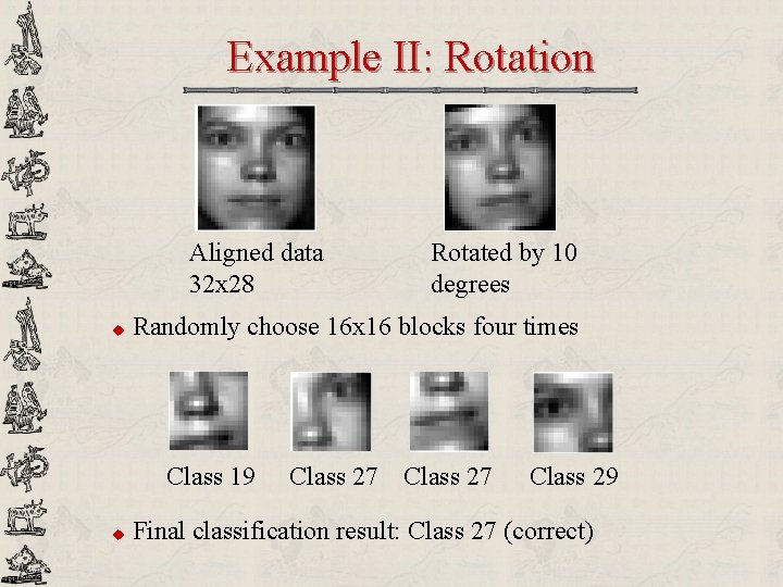
Example II: Rotation Aligned data 32 x 28 u Randomly choose 16 x 16 blocks four times Class 19 u Rotated by 10 degrees Class 27 Class 29 Final classification result: Class 27 (correct)

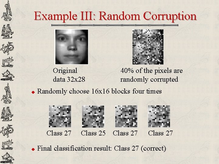
Example III: Random Corruption Original data 32 x 28 u Randomly choose 16 x 16 blocks four times Class 27 u 40% of the pixels are randomly corrupted Class 25 Class 27 Final classification result: Class 27 (correct)

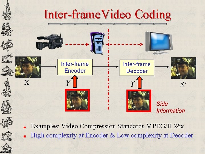
Inter-frame. Video Coding Inter-frame Encoder X Inter-frame Decoder X’ Side Information Examples: Video Compression Standards MPEG/H. 26 x High complexity at Encoder & Low complexity at Decoder

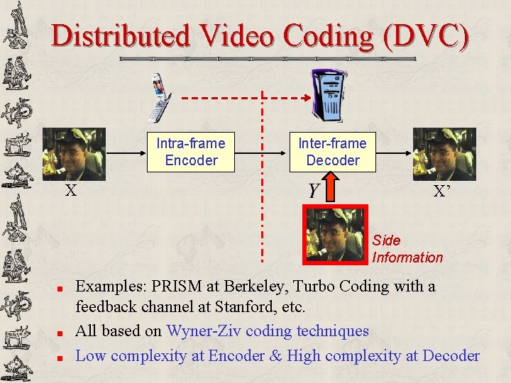
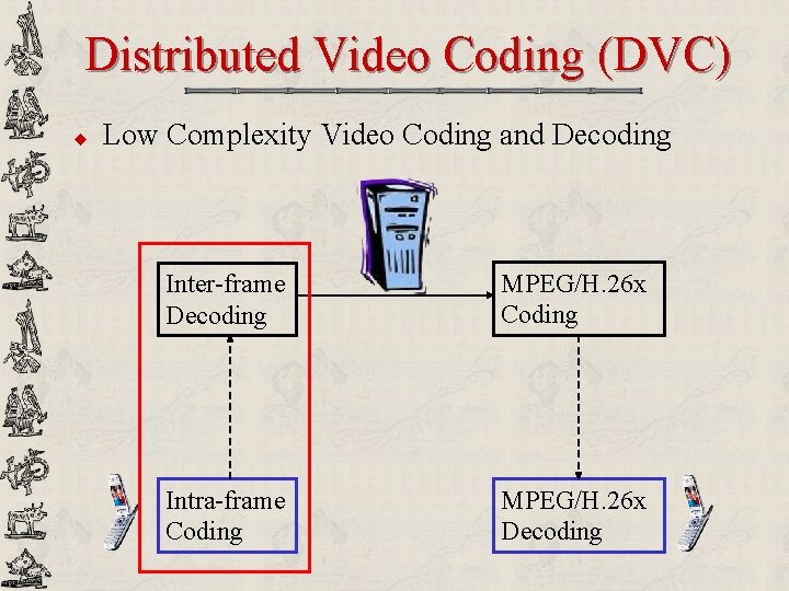
Distributed Video Coding (DVC) Intra-frame Encoder X Inter-frame Decoder X’ Side Information Examples: PRISM at Berkeley, Turbo Coding with a feedback channel at Stanford, etc. All based on Wyner-Ziv coding techniques Low complexity at Encoder & High complexity at Decoder

Distributed Video Coding (DVC) u Low Complexity Video Coding and Decoding Inter-frame Decoding MPEG/H. 26 x Coding Intra-frame Coding MPEG/H. 26 x Decoding

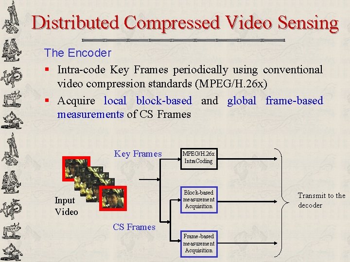
Distributed Compressed Video Sensing The Encoder § Intra-code Key Frames periodically using conventional video compression standards (MPEG/H. 26 x) § Acquire local block-based and global frame-based measurements of CS Frames Key Frames MPEG/H. 26 x Intra. Coding Block-based measurement Acquisition Input Video CS Frames Frame-based measurement Acquisition Transmit to the decoder

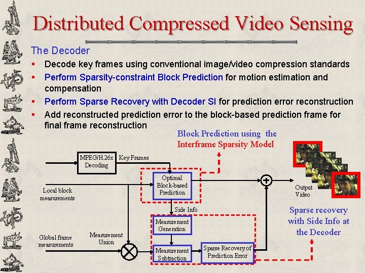
Distributed Compressed Video Sensing The Decoder § § Decode key frames using conventional image/video compression standards Perform Sparsity-constraint Block Prediction for motion estimation and compensation Perform Sparse Recovery with Decoder SI for prediction error reconstruction Add reconstructed prediction error to the block-based prediction frame for final frame reconstruction Block Prediction using the Interframe Sparsity Model MPEG/H. 26 x Key Frames Decoding Optimal Block-based Prediction Local block measurements Output Video Sparse recovery with Side Info at the Decoder Side Info Global frame measurements Measurement Union Measurement Generation Measurement Subtraction Sparse Recovery of Prediction Error

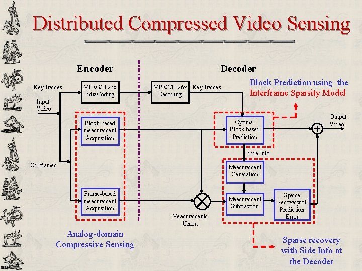
Distributed Compressed Video Sensing Encoder Key-frames MPEG/H. 26 x Intra. Coding Decoder MPEG/H. 26 x Key-frames Decoding Block Prediction using the Interframe Sparsity Model Input Video Output Video Optimal Block-based Prediction Block-based measurement Acquisition Side Info CS-frames Measurement Generation Frame-based measurement Acquisition Measurement Subtraction Measurements Union Analog-domain Compressive Sensing Sparse Recovery of Prediction Error Sparse recovery with Side Info at the Decoder

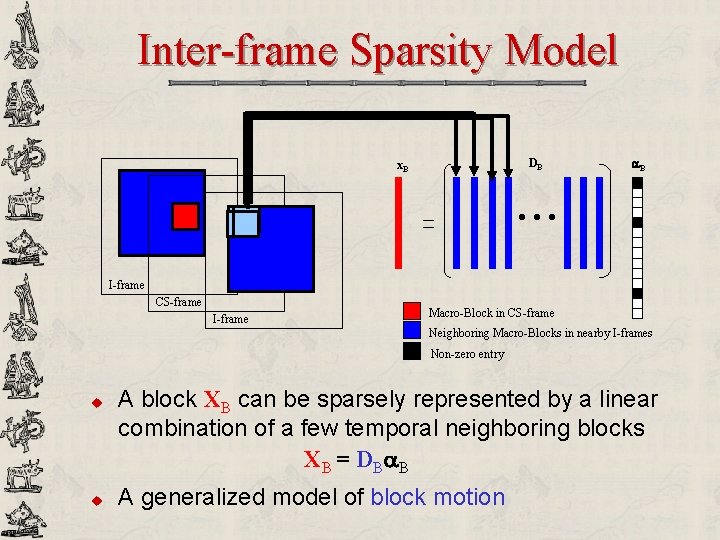
Inter-frame Sparsity Model DB x. B B • • • I-frame CS-frame I-frame Macro-Block in CS-frame Neighboring Macro-Blocks in nearby I-frames Non-zero entry u u A block XB can be sparsely represented by a linear combination of a few temporal neighboring blocks XB = DB B A generalized model of block motion

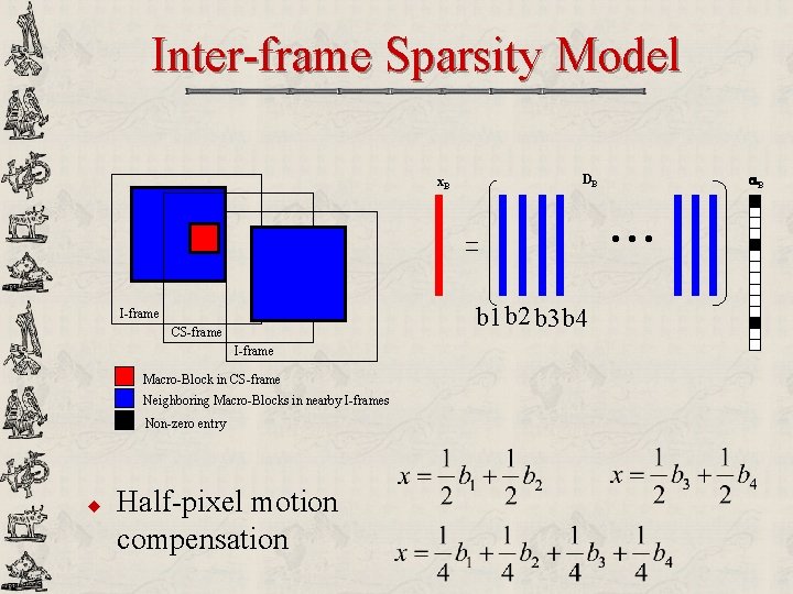
Inter-frame Sparsity Model x. B B DB • • • b 1 b 2 b 3 b 4 I-frame CS-frame I-frame Macro-Block in CS-frame Neighboring Macro-Blocks in nearby I-frames Non-zero entry u Half-pixel motion compensation

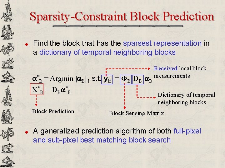
Sparsity-Constraint Block Prediction u Find the block that has the sparsest representation in a dictionary of temporal neighboring blocks *B = Argmin | B|1 s. t. y. B = ΦB DB B X*B = DB *B Block Prediction u Received local block measurements Dictionary of temporal neighboring blocks Block Sensing Matrix A generalized prediction algorithm of both full-pixel and sub-pixel best matching block search

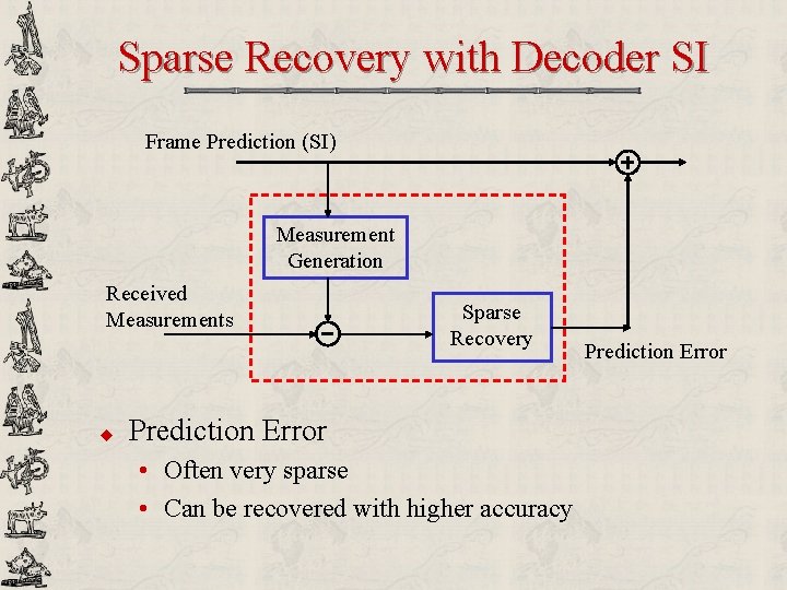
Sparse Recovery with Decoder SI Frame Prediction (SI) Measurement Generation Received Measurements u Sparse Recovery Prediction Error • Often very sparse • Can be recovered with higher accuracy Prediction Error

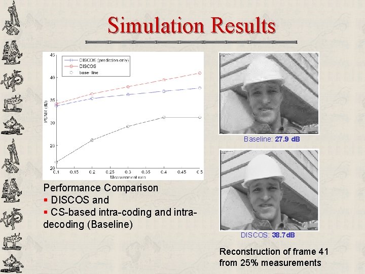
Simulation Results Baseline: 27. 9 d. B Performance Comparison § DISCOS and § CS-based intra-coding and intradecoding (Baseline) DISCOS: 38. 7 d. B Reconstruction of frame 41 from 25% measurements

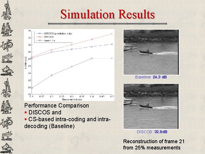
Simulation Results Baseline: 24. 3 d. B Performance Comparison § DISCOS and § CS-based intra-coding and intradecoding (Baseline) DISCOS: 32. 9 d. B Reconstruction of frame 21 from 25% measurements

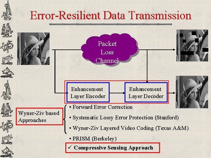
Error-Resilient Data Transmission Packet Loss Channel Enhancement Layer Encoder Wyner-Ziv based Approaches Enhancement Layer Decoder • Forward Error Correction • Systematic Lossy Error Protection (Stanford) • Wyner-Ziv Layered Video Coding (Texas A&M) • PRISM (Berkeley) ü Compressive Sensing Approach

Previous Approaches u FEC § Employ well-known channel codes (Reed-Solomon, Turbo code or LDPC, etc) § Decoded video quality significantly degraded when packet loss rate higher than error correction capacity of the channel code (cliff effect) All based on coding technique on a finite field u Recent Approaches § Wyner-Ziv coding technique based: SLEP (Stanford), Layered Wyner-Ziv Video Coding (Texas A&M) § Distributed Video Coding to mitigate error propagation of the predictive video coding: PRISM (Berkeley)

Compressive Sensing Approach A new channel-coding technique on a REAL FIELD u u u Borrow principles from Compressive Sensing Effectively mitigate the cliff effect thanks to the soft-decoding feature of Sparse Recovery Algorithm Eliminate “Get all or nothing” feature of coding techniques on a finite field

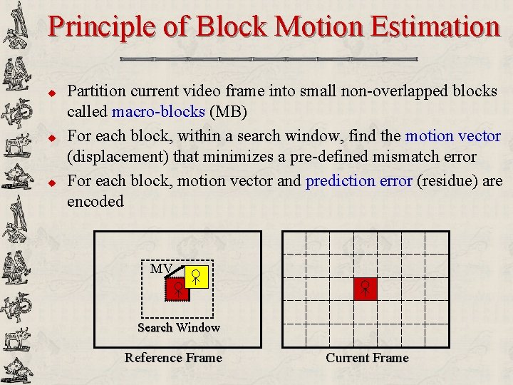
Principle of Block Motion Estimation u u u Partition current video frame into small non-overlapped blocks called macro-blocks (MB) For each block, within a search window, find the motion vector (displacement) that minimizes a pre-defined mismatch error For each block, motion vector and prediction error (residue) are encoded MV Search Window Reference Frame Current Frame

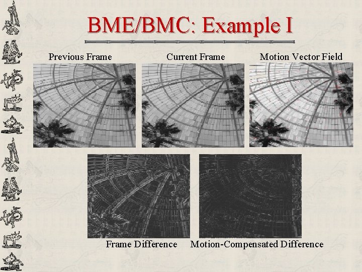
BME/BMC: Example I Previous Frame Current Frame Difference Motion Vector Field Motion-Compensated Difference

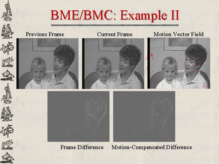
BME/BMC: Example II Previous Frame Current Frame Difference Motion Vector Field Motion-Compensated Difference

Compressive Sensing Overview Measurement vector Sensing matrix Sparsifying matrix Sparse transform coefficients Input signal Sparse Recovery: * = Argmin | |1 s. t. y = ΦΨ X* = Ψ *

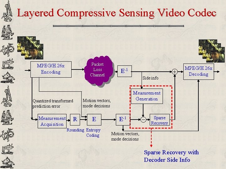
Layered Compressive Sensing Video Codec Packet Loss Channel MPEG/H. 26 x Encoding Quantized transformed prediction error Measurement Acquisition R E-1 Side info Measurement Generation Motion vectors, mode decisions E Rounding Entropy Coding MPEG/H. 26 x Decoding E-1 Sparse Recovery Motion vectors, mode decisions Sparse Recovery with Decoder Side Info

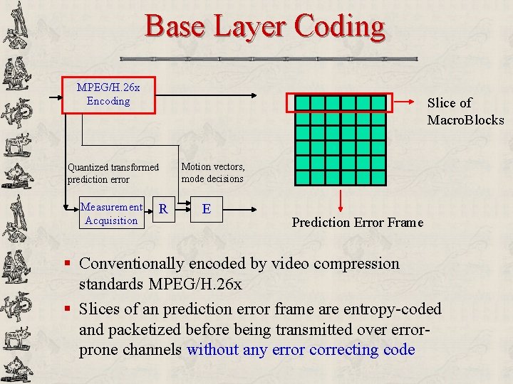
Base Layer Coding MPEG/H. 26 x Encoding Slice of Macro. Blocks Quantized transformed prediction error Measurement Acquisition R Motion vectors, mode decisions E Prediction Error Frame § Conventionally encoded by video compression standards MPEG/H. 26 x § Slices of an prediction error frame are entropy-coded and packetized before being transmitted over errorprone channels without any error correcting code

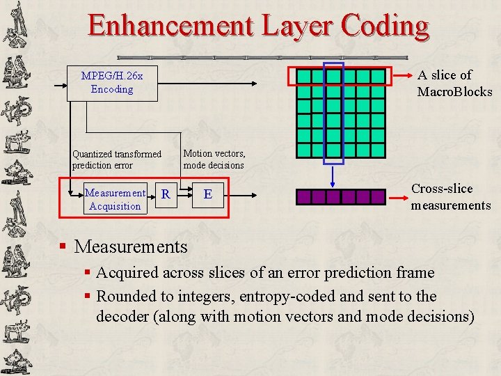
Enhancement Layer Coding A slice of Macro. Blocks MPEG/H. 26 x Encoding Quantized transformed prediction error Measurement Acquisition Motion vectors, mode decisions R E Cross-slice measurements § Measurements § Acquired across slices of an error prediction frame § Rounded to integers, entropy-coded and sent to the decoder (along with motion vectors and mode decisions)

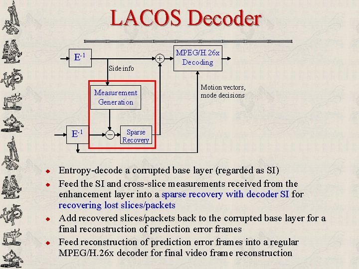
LACOS Decoder E-1 Side info Measurement Generation E-1 u u MPEG/H. 26 x Decoding Motion vectors, mode decisions Sparse Recovery Entropy-decode a corrupted base layer (regarded as SI) Feed the SI and cross-slice measurements received from the enhancement layer into a sparse recovery with decoder SI for recovering lost slices/packets Add recovered slices/packets back to the corrupted base layer for a final reconstruction of prediction error frames Feed reconstruction of prediction error frames into a regular MPEG/H. 26 x decoder for final video frame reconstruction

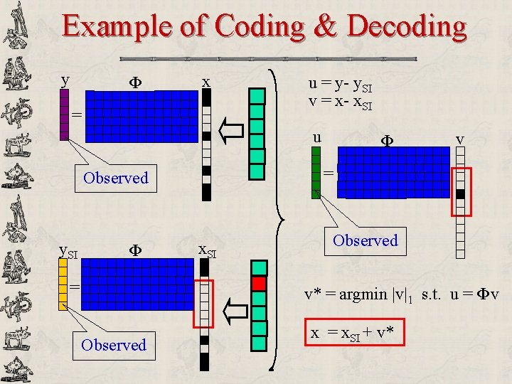
Example of Coding & Decoding y Φ x = u = y- y. SI v = x- x. SI u Φ = v = Observed y. SI Φ x. SI Observed v* = argmin |v|1 s. t. u = Φv Observed x = x. SI + v*

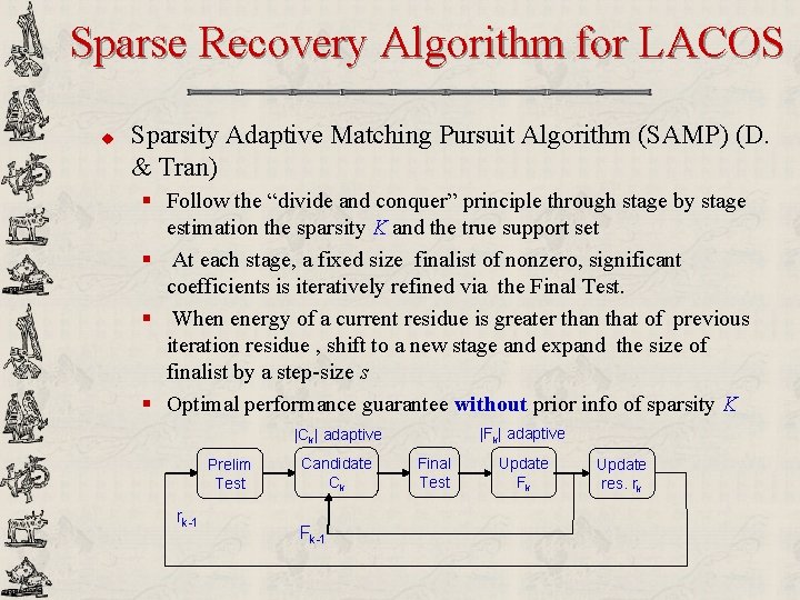
Sparse Recovery Algorithm for LACOS u Sparsity Adaptive Matching Pursuit Algorithm (SAMP) (D. & Tran) § Follow the “divide and conquer” principle through stage by stage estimation the sparsity K and the true support set § At each stage, a fixed size finalist of nonzero, significant coefficients is iteratively refined via the Final Test. § When energy of a current residue is greater than that of previous iteration residue , shift to a new stage and expand the size of finalist by a step-size s § Optimal performance guarantee without prior info of sparsity K |Fk| adaptive |Ck| adaptive Prelim Test rk-1 Candidate Ck Fk-1 Final Test Update Fk Update res. rk

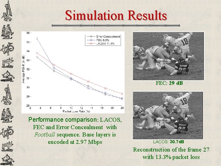
Simulation Results FEC: 29 d. B Performance comparison: LACOS, FEC and Error Concealment with Football sequence. Base layers is encoded at 2. 97 Mbps LACOS: 30. 7 d. B Reconstruction of the frame 27 with 13. 3% packet loss

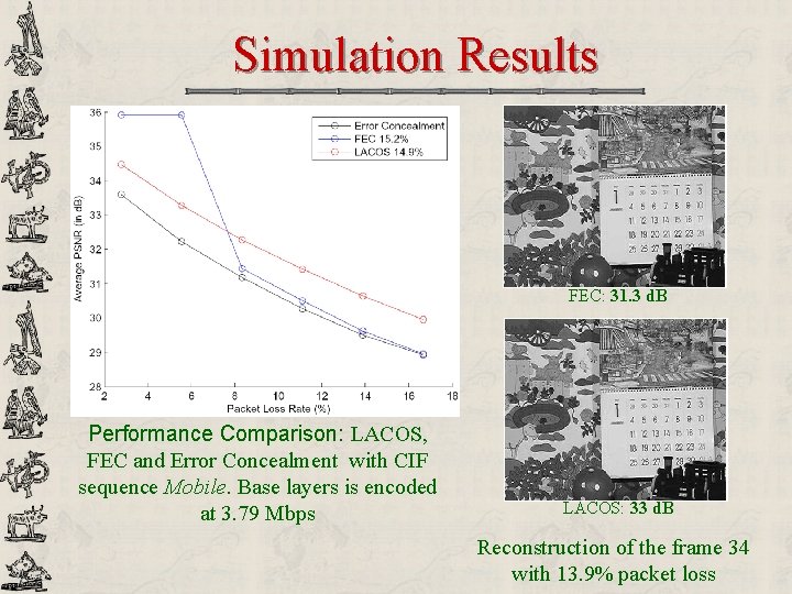
Simulation Results FEC: 31. 3 d. B Performance Comparison: LACOS, FEC and Error Concealment with CIF sequence Mobile. Base layers is encoded at 3. 79 Mbps LACOS: 33 d. B Reconstruction of the frame 34 with 13. 9% packet loss

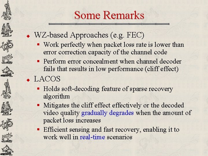
Some Remarks u WZ-based Approaches (e. g. FEC) § Work perfectly when packet loss rate is lower than error correction capacity of the channel code § Perform error concealment when channel decoder fails that results in low performance (cliff effect) u LACOS § Holds soft-decoding feature of sparse recovery algorithm § Mitigates the cliff effectively or the decoded video quality gradually degrades when the amount of packet loss increases § Efficient sensing and fast recovery, enabling it to work well in real-time scenarios

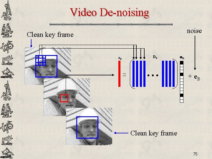
Video De-noising noise Clean key frame x. B DB • • • B + e. B Clean key frame 75

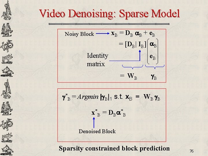
Video Denoising: Sparse Model Noisy Block x. B = DB B + e. B = [DB| IB] B Identity matrix e. B = WB B *B = Argmin | B|1 s. t. x. B = WB B x*B = DB *B Denoised Block Sparsity constrained block prediction 76

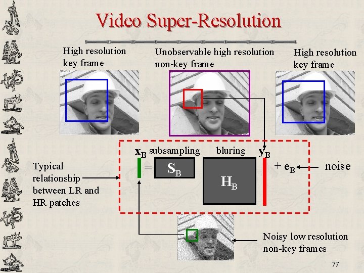
Video Super-Resolution High resolution key frame Typical relationship between LR and HR patches Unobservable high resolution non-key frame x. B subsampling = SB bluring HB y. B High resolution key frame + e. B noise Noisy low resolution non-key frames 77

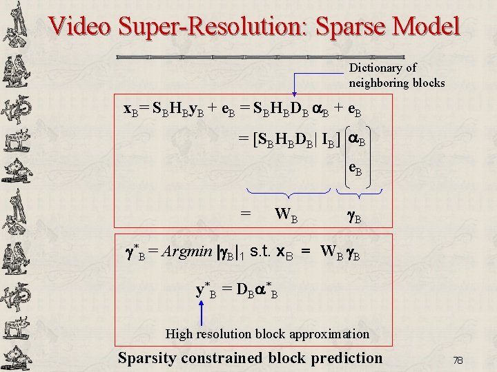
Video Super-Resolution: Sparse Model Dictionary of neighboring blocks x. B= SBHBy. B + e. B = SBHBDB B + e. B = [SBHBDB| IB] B e. B = WB B *B = Argmin | B|1 s. t. x. B = WB B y*B = DB *B High resolution block approximation Sparsity constrained block prediction 78

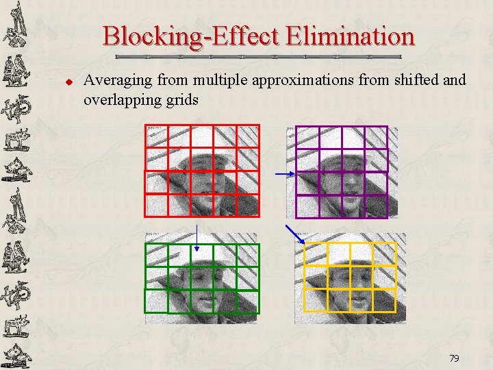
Blocking-Effect Elimination u Averaging from multiple approximations from shifted and overlapping grids 79

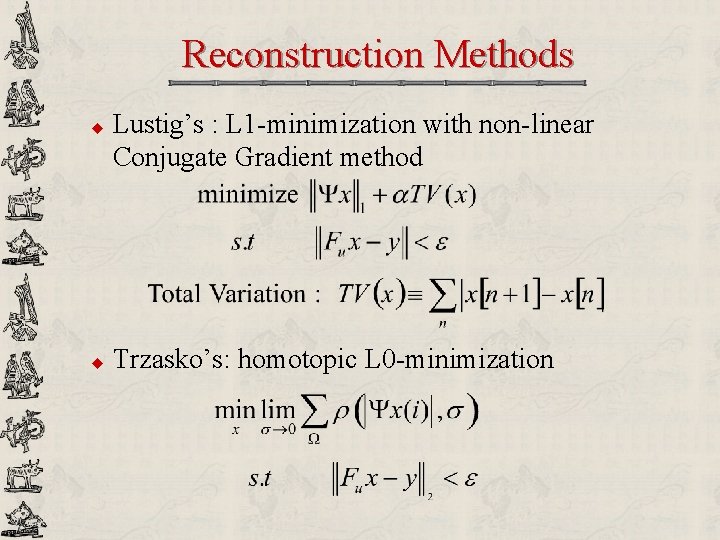
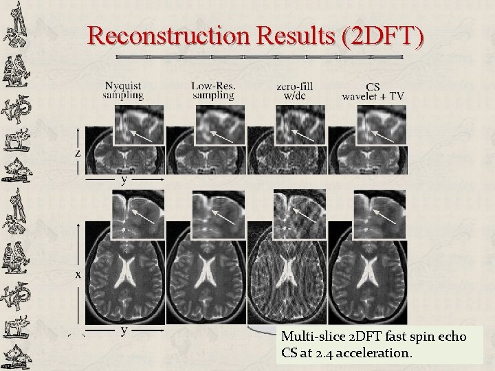
Compressed Sensing in Medical Imaging u Goal so far: § Achieve faster MR imaging while maintaining reconstruction quality u Methods: § under sample discrete Fourier space using some pseudo-random patterns § then reconstruct using L 1 -minimization (Lustig) or homotopic L 0 -minimization (Trzasko)

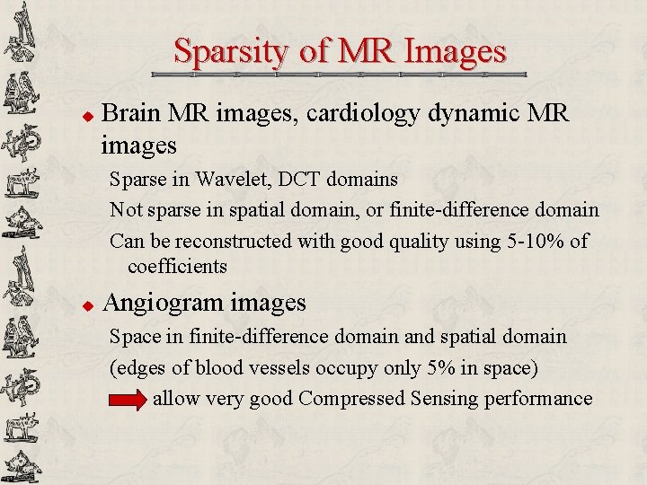
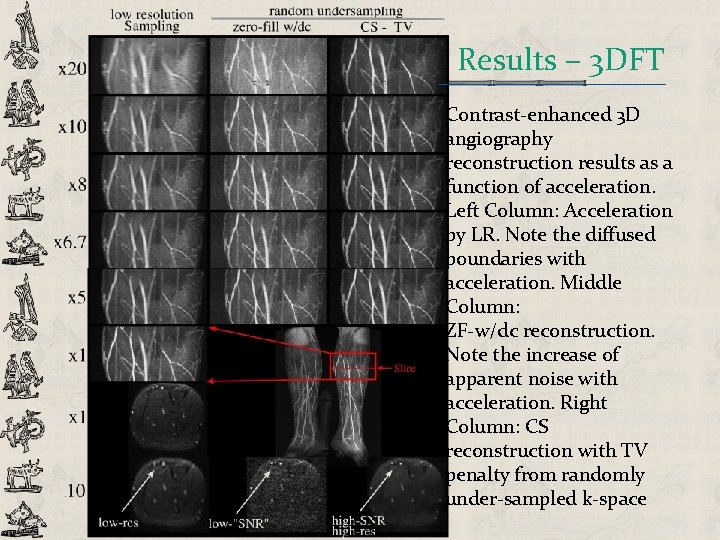
Sparsity of MR Images u Brain MR images, cardiology dynamic MR images Sparse in Wavelet, DCT domains Not sparse in spatial domain, or finite-difference domain Can be reconstructed with good quality using 5 -10% of coefficients u Angiogram images Space in finite-difference domain and spatial domain (edges of blood vessels occupy only 5% in space) allow very good Compressed Sensing performance

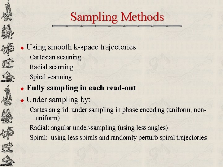
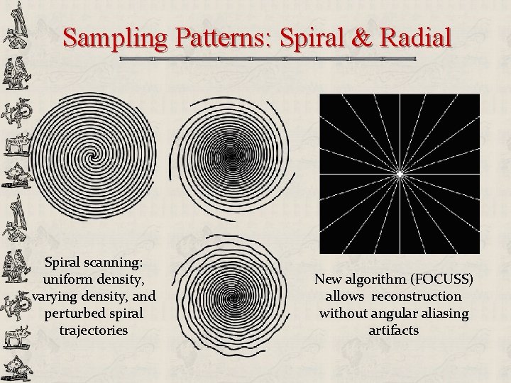
Sampling Methods u Using smooth k-space trajectories Cartesian scanning Radial scanning Spiral scanning u u Fully sampling in each read-out Under sampling by: Cartesian grid: under sampling in phase encoding (uniform, nonuniform) Radial: angular under-sampling (using less angles) Spiral: using less spirals and randomly perturb spiral trajectories

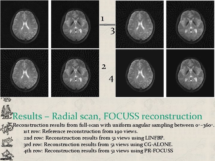
Sampling Patterns: Spiral & Radial Spiral scanning: uniform density, varying density, and perturbed spiral trajectories New algorithm (FOCUSS) allows reconstruction without angular aliasing artifacts

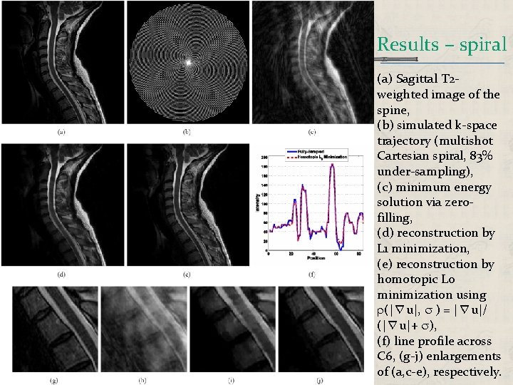
Reconstruction Methods u u Lustig’s : L 1 -minimization with non-linear Conjugate Gradient method Trzasko’s: homotopic L 0 -minimization

Reconstruction Results (2 DFT) Multi-slice 2 DFT fast spin echo CS at 2. 4 acceleration.

Results – 3 DFT Contrast-enhanced 3 D angiography reconstruction results as a function of acceleration. Left Column: Acceleration by LR. Note the diffused boundaries with acceleration. Middle Column: ZF-w/dc reconstruction. Note the increase of apparent noise with acceleration. Right Column: CS reconstruction with TV penalty from randomly under-sampled k-space

1 2 3 4 Results – Radial scan, FOCUSS reconstruction Reconstruction results from full-scan with uniform angular sampling between 0◦– 360◦. 1 st row: Reference reconstruction from 190 views. 2 nd row: Reconstruction results from 51 views using LINFBP. 3 rd row: Reconstruction results from 51 views using CG-ALONE. 4 th row: Reconstruction results from 51 views using PR-FOCUSS

Results – spiral (a) Sagittal T 2 weighted image of the spine, (b) simulated k-space trajectory (multishot Cartesian spiral, 83% under-sampling), (c) minimum energy solution via zerofilling, (d) reconstruction by L 1 minimization, (e) reconstruction by homotopic L 0 minimization using (|∇u|, ) = |∇u|/ (|∇u|+ ), (f) line profile across C 6, (g-j) enlargements of (a, c-e), respectively.

Conclusion u Compressed sensing § § § u A different paradigm for data acquisition Sample less and compute more Simple encoding; most computation at decoder Exploit a priori signal sparsity Universality, robustness Compressed sensing applications for multimedia § § § 2 D separable measurement ensemble for image/video Face/speech recognition Distributed compressed video sensing Layered robust video transmission Image/Video De-noising & Concealment MRI applications

References u u http: //www. dsp. ece. rice. edu/cs/ http: //nuitblanche. blogspot. com/search/label/compressed%20 sensing