Complexity Analysis of Data Structures Algorithms Piyush Kumar

Complexity & Analysis of Data Structures & Algorithms Piyush Kumar (Lecture 2: Algorithmic Analysis) Welcome to COP 4531 Based on slides from J. Edmonds, S. Rudich, S. H. Teng, K. Wayne and my old slides.

Algorithm: What is it? • An Algorithm a well-defined computational procedure that transforms inputs into outputs, achieving the desired input-output relationship.

Algorithm Characteristics • • Finiteness Input Correctness Output Rigorous, Unambiguous and Sufficiently Basic at each step

Applications? • • • WWW and the Internet Computational Biology Scientific Simulation VLSI Design Security Automated Vision/Image Processing Compression of Databases Mathematical Optimization

Sorting • Input: Array A[1. . . n], of elements in arbitrary order • Output: Array A[1. . . n] of the same elements, but in increasing order • Given a teacher find all his/her students. • Given a student find all his/her teachers.

The RAM Model • Analysis is performed with respect to a computational model • We will usually use a generic uniprocessor random-access machine (RAM) – All memory equally expensive to access – No concurrent operations – All reasonable instructions take unit time • Except, of course, function calls – Constant word size • Unless we are explicitly manipulating bits

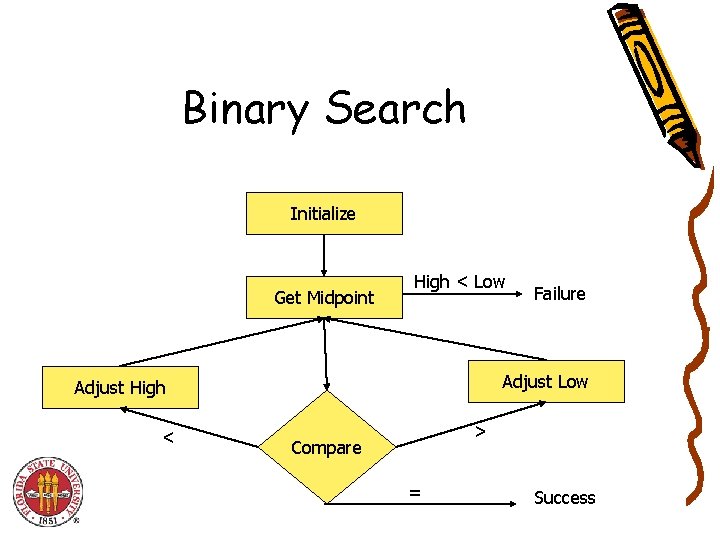
Binary Search Initialize Get Midpoint High < Low Adjust High < Failure > Compare = Success

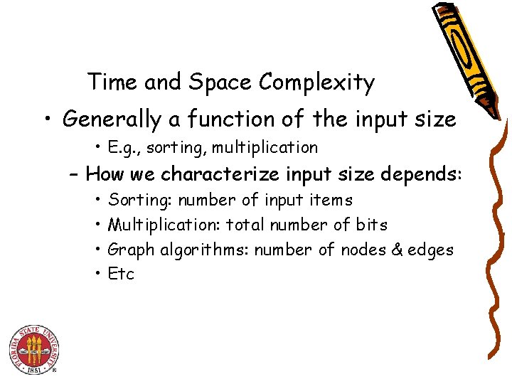
Time and Space Complexity • Generally a function of the input size • E. g. , sorting, multiplication – How we characterize input size depends: • • Sorting: number of input items Multiplication: total number of bits Graph algorithms: number of nodes & edges Etc

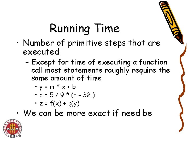
Running Time • Number of primitive steps that are executed – Except for time of executing a function call most statements roughly require the same amount of time • y=m*x+b • c = 5 / 9 * (t - 32 ) • z = f(x) + g(y) • We can be more exact if need be

Analysis • Worst case – Provides an upper bound on running time – An absolute guarantee • Average case – Provides the expected running time – Very useful, but treat with care: what is “average”? • Random (equally likely) inputs • Real-life inputs

Binary Search Analysis • • Order Notation Upper Bounds Search Time = ? ? A better way to look at it, Binary Search Trees

In this course • We care most about asymptotic performance – How does the algorithm behave as the problem size gets very large? • Running time • Memory/storage requirements • Bandwidth/power requirements/logic gates/etc.

2. 1 Computational Tractability "For me, great algorithms are the poetry of computation. Just like verse, they can be terse, allusive, dense, and even mysterious. But once unlocked, they cast a brilliant new light on some aspect of computing. " - Francis Sullivan

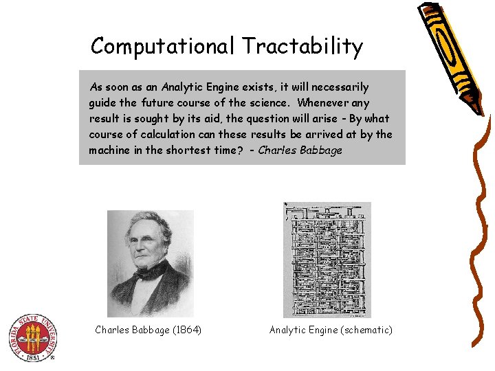
Computational Tractability As soon as an Analytic Engine exists, it will necessarily guide the future course of the science. Whenever any result is sought by its aid, the question will arise - By what course of calculation can these results be arrived at by the machine in the shortest time? - Charles Babbage (1864) Analytic Engine (schematic)

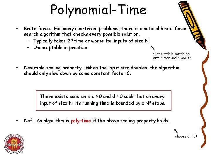
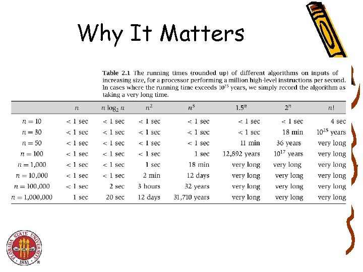
Polynomial-Time • Brute force. For many non-trivial problems, there is a natural brute force search algorithm that checks every possible solution. – Typically takes 2 N time or worse for inputs of size N. – Unacceptable in practice. n ! for stable matching with n men and n women • Desirable scaling property. When the input size doubles, the algorithm should only slow down by some constant factor C. There exists constants c > 0 and d > 0 such that on every input of size N, its running time is bounded by c Nd steps. • Def. An algorithm is poly-time if the above scaling property holds. choose C = 2 d

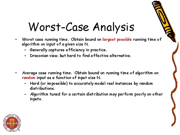
Worst-Case Analysis • Worst case running time. Obtain bound on largest possible running time of algorithm on input of a given size N. – Generally captures efficiency in practice. – Draconian view, but hard to find effective alternative. • Average case running time. Obtain bound on running time of algorithm on random input as a function of input size N. – Hard (or impossible) to accurately model real instances by random distributions. – Algorithm tuned for a certain distribution may perform poorly on other inputs.

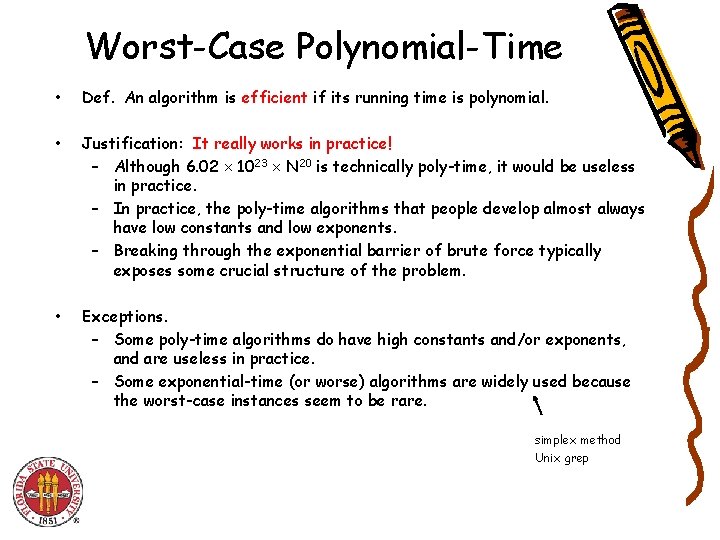
Worst-Case Polynomial-Time • Def. An algorithm is efficient if its running time is polynomial. • Justification: It really works in practice! – Although 6. 02 1023 N 20 is technically poly-time, it would be useless in practice. – In practice, the poly-time algorithms that people develop almost always have low constants and low exponents. – Breaking through the exponential barrier of brute force typically exposes some crucial structure of the problem. • Exceptions. – Some poly-time algorithms do have high constants and/or exponents, and are useless in practice. – Some exponential-time (or worse) algorithms are widely used because the worst-case instances seem to be rare. simplex method Unix grep

Why It Matters

2. 2 Asymptotic Order of Growth

Why not do Exact Analysis? • It is difficult to be exact. • Results are most of the time too complicated and irrelevant.

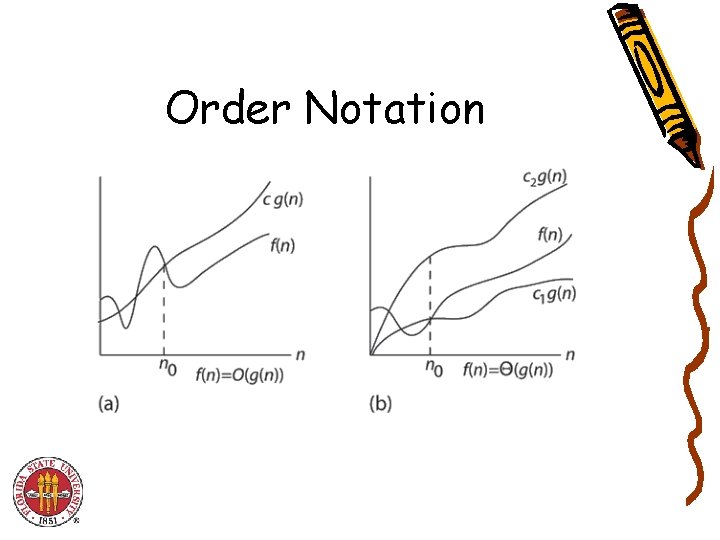
Order Notation

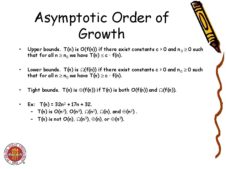
Asymptotic Order of Growth • Upper bounds. T(n) is O(f(n)) if there exist constants c > 0 and n 0 0 such that for all n n 0 we have T(n) c · f(n). • Lower bounds. T(n) is (f(n)) if there exist constants c > 0 and n 0 0 such that for all n n 0 we have T(n) c · f(n). • Tight bounds. T(n) is (f(n)) if T(n) is both O(f(n)) and (f(n)). • Ex: T(n) = 32 n 2 + 17 n + 32. – T(n) is O(n 2), O(n 3), (n 2), (n), and (n 2). – T(n) is not O(n), (n 3), (n), or (n 3).

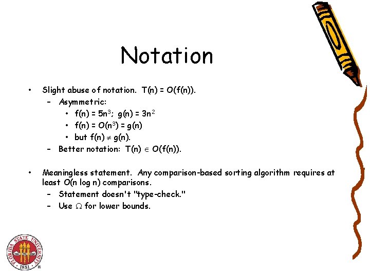
Notation • Slight abuse of notation. T(n) = O(f(n)). – Asymmetric: • f(n) = 5 n 3; g(n) = 3 n 2 • f(n) = O(n 3) = g(n) • but f(n) g(n). – Better notation: T(n) O(f(n)). • Meaningless statement. Any comparison-based sorting algorithm requires at least O(n log n) comparisons. – Statement doesn't "type-check. " – Use for lower bounds.

Properties • Transitivity. – If f = O(g) and g = O(h) then f = O(h). – If f = (g) and g = (h) then f = (h). • Additivity. – If f = O(h) and g = O(h) then f + g = O(h). – If f = (h) and g = (h) then f + g = (h). – If f = (h) and g = O(h) then f + g = (h).

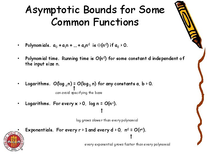
Asymptotic Bounds for Some Common Functions • Polynomials. a 0 + a 1 n + … + adnd is (nd) if ad > 0. • Polynomial time. Running time is O(nd) for some constant d independent of the input size n. • Logarithms. O(log a n) = O(log b n) for any constants a, b > 0. can avoid specifying the base • Logarithms. For every x > 0, log n = O(nx). log grows slower than every polynomial • Exponentials. For every r > 1 and every d > 0, nd = O(rn). every exponential grows faster than every polynomial

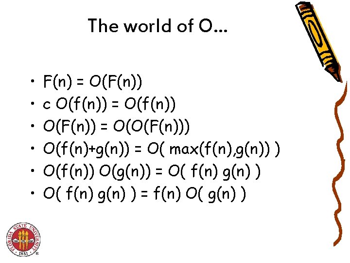
The world of O… • • • F(n) = O(F(n)) c O(f(n)) = O(f(n)) O(F(n)) = O(O(F(n))) O(f(n)+g(n)) = O( max(f(n), g(n)) ) O(f(n)) O(g(n)) = O( f(n) g(n) ) = f(n) O( g(n) )

2. 4 A Survey of Common Running Times

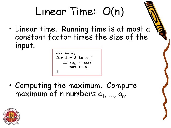
Linear Time: O(n) • Linear time. Running time is at most a constant factor times the size of the input. max a 1 for i = 2 to n { if (ai > max) max ai } • Computing the maximum. Compute maximum of n numbers a 1, …, an.

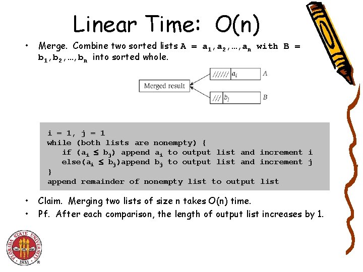
Linear Time: O(n) • Merge. Combine two sorted lists A = a 1, a 2, …, an with B = b 1, b 2, …, bn into sorted whole. i = 1, j = 1 while (both lists are nonempty) { if (ai bj) append ai to output list and increment i else(ai bj)append bj to output list and increment j } append remainder of nonempty list to output list • • Claim. Merging two lists of size n takes O(n) time. Pf. After each comparison, the length of output list increases by 1.

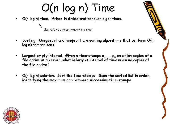
O(n log n) Time • O(n log n) time. Arises in divide-and-conquer algorithms. also referred to as linearithmic time • Sorting. Mergesort and heapsort are sorting algorithms that perform O(n log n) comparisons. • Largest empty interval. Given n time-stamps x 1, …, xn on which copies of a file arrive at a server, what is largest interval of time when no copies of the file arrive? • O(n log n) solution. Sort the time-stamps. Scan the sorted list in order, identifying the maximum gap between successive time-stamps.

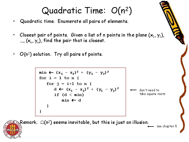
Quadratic Time: O(n 2) • Quadratic time. Enumerate all pairs of elements. • Closest pair of points. Given a list of n points in the plane (x 1, y 1), …, (xn, yn), find the pair that is closest. • O(n 2) solution. Try all pairs of points. min (x 1 - x 2)2 + (y 1 - y 2)2 for i = 1 to n { for j = i+1 to n { d (xi - xj)2 + (yi - yj)2 if (d < min) min d } } • don't need to take square roots Remark. (n 2) seems inevitable, but this is just an illusion. see chapter 5

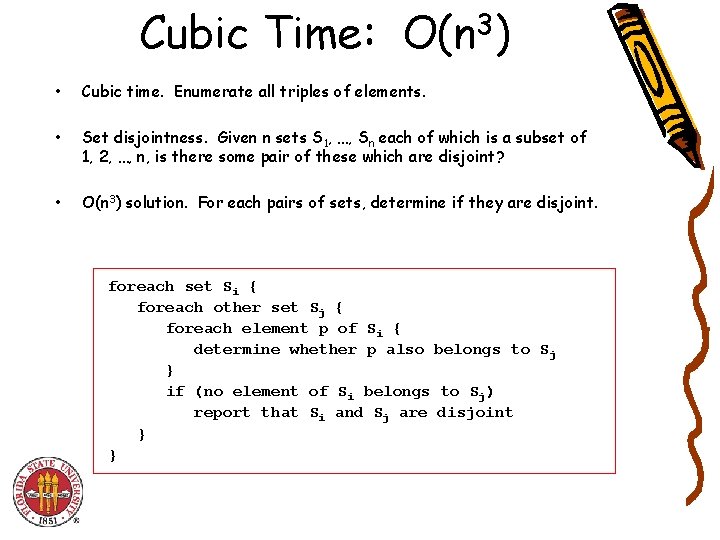
Cubic Time: 3 O(n ) • Cubic time. Enumerate all triples of elements. • Set disjointness. Given n sets S 1, …, Sn each of which is a subset of 1, 2, …, n, is there some pair of these which are disjoint? • O(n 3) solution. For each pairs of sets, determine if they are disjoint. foreach set Si { foreach other set Sj { foreach element p of Si { determine whether p also belongs to Sj } if (no element of Si belongs to Sj) report that Si and Sj are disjoint } }

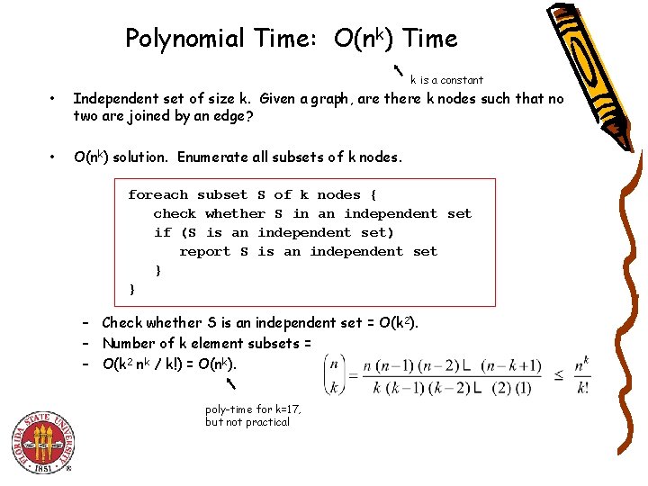
Polynomial Time: O(nk) Time k is a constant • Independent set of size k. Given a graph, are there k nodes such that no two are joined by an edge? • O(nk) solution. Enumerate all subsets of k nodes. foreach subset S of k nodes { check whether S in an independent set if (S is an independent set) report S is an independent set } } – Check whether S is an independent set = O(k 2). – Number of k element subsets = – O(k 2 nk / k!) = O(nk). poly-time for k=17, but not practical

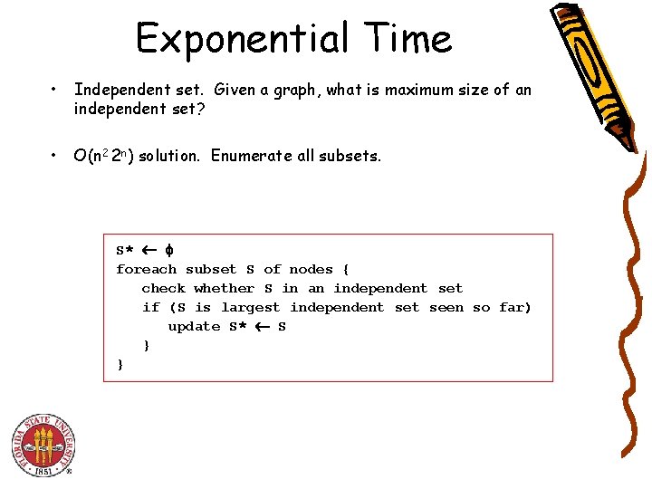
Exponential Time • Independent set. Given a graph, what is maximum size of an independent set? • O(n 2 2 n) solution. Enumerate all subsets. S* foreach subset S of nodes { check whether S in an independent set if (S is largest independent seen so far) update S* S } }

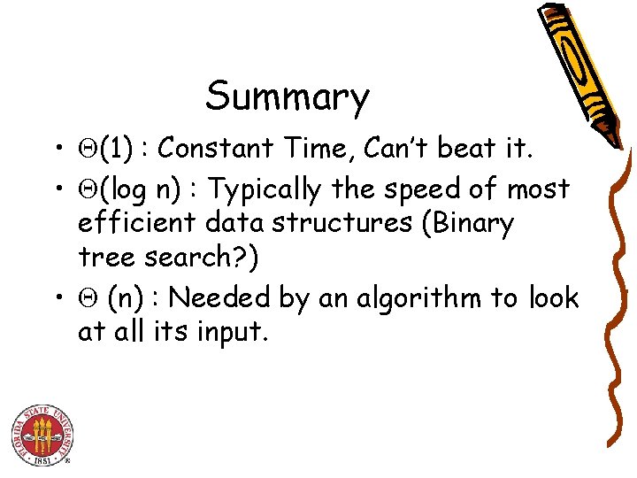
Summary • (1) : Constant Time, Can’t beat it. • (log n) : Typically the speed of most efficient data structures (Binary tree search? ) • (n) : Needed by an algorithm to look at all its input.

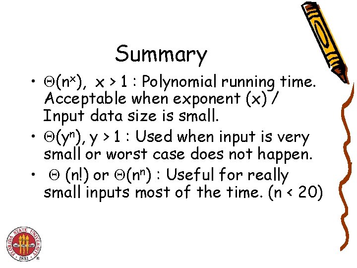
Summary • (nx), x > 1 : Polynomial running time. Acceptable when exponent (x) / Input data size is small. • (yn), y > 1 : Used when input is very small or worst case does not happen. • (n!) or (nn) : Useful for really small inputs most of the time. (n < 20)

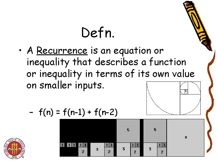
Defn. • A Recurrence is an equation or inequality that describes a function or inequality in terms of its own value on smaller inputs. – f(n) = f(n-1) + f(n-2)

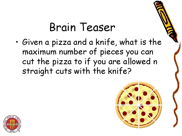
Brain Teaser • Given a pizza and a knife, what is the maximum number of pieces you can cut the pizza to if you are allowed n straight cuts with the knife?