Complex Regression Models NonLinear Relationships Polynomial Regression Data

Complex Regression Models Non-Linear Relationships Polynomial Regression Data Transforms Quadratic and Interaction Terms

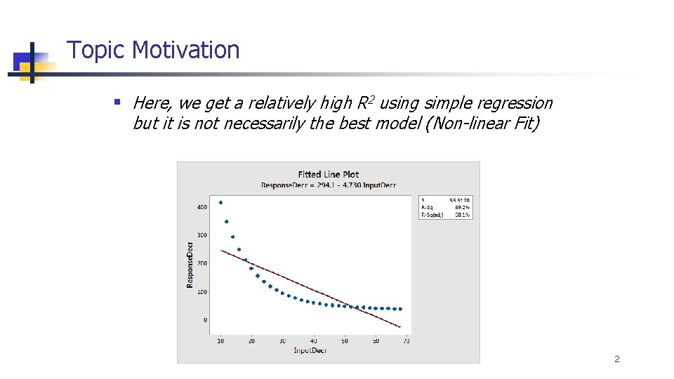
Topic Motivation § Here, we get a relatively high R 2 using simple regression but it is not necessarily the best model (Non-linear Fit) 2

Topics I. Linear vs. Non-Linear ‘Models’ II. Polynomial Regression with Quadratic Terms III. Log Transforms IV. Models with Interaction Terms Appendix – Binary Logistic Regression with Quadratic Terms and Interactions 3

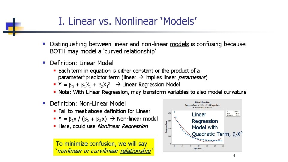
I. Linear vs. Nonlinear ‘Models’ § Distinguishing between linear and non-linear models is confusing because BOTH may model a ‘curved relationship’ § Definition: Linear Model § Each term in equation is either constant or the product of a parameter*predictor term (linear implies linear parameters) § Y = b 0 + b 1 X 1 + b 2 X 12 Linear Regression Model § Note: With Linear Regression, may transform variables to also model curvature § Definition: Non-Linear Model § Fail to meet above definition for Linear § Y = b 1 x / (b 0 + b 2 x) Non-linear model § Here, could use Nonlinear Regression To minimize confusion, we will say ‘nonlinear or curvilinear relationship’ Linear Regression Model with Quadratic Term, b 2 X 2 4

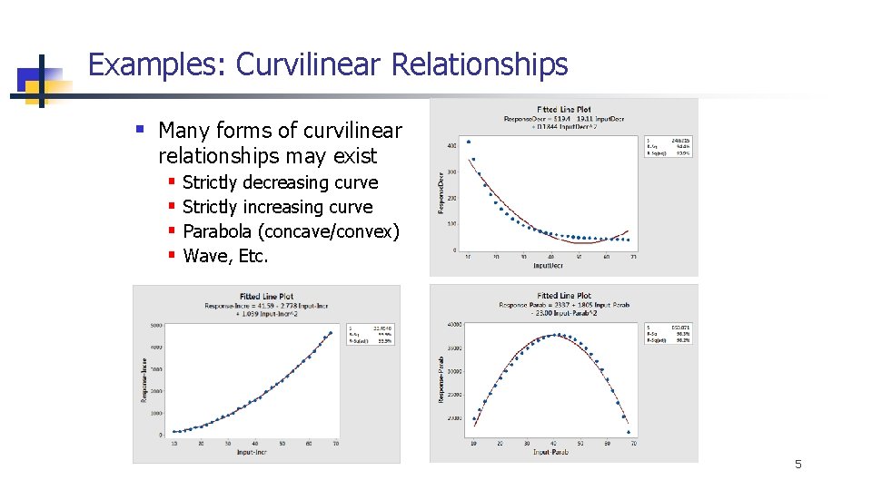
Examples: Curvilinear Relationships § Many forms of curvilinear relationships may exist § § Strictly decreasing curve Strictly increasing curve Parabola (concave/convex) Wave, Etc. 5

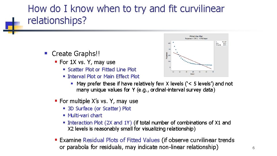
How do I know when to try and fit curvilinear relationships? § Create Graphs!! § For 1 X vs. Y, may use § Scatter Plot or Fitted Line Plot § Interval Plot or Main Effect Plot § May prefer these if have relatively few X levels (‘< 5 levels’) and not many unique values for Y (e. g. , ordinal-interval survey data) § For multiple X’s vs. Y, may use § 3 D Surface (or Scatter) Plot § Multi-vari chart § Interaction Plot (2 X and 1 Y) (if total number of combinations of X 1 and X 2 levels is reasonably small for visualizing relationship) § Examine Residual Plots of Fitted Values (if observe curvilinear trends or parabola for residuals, may indicate non-linear relationship) 6

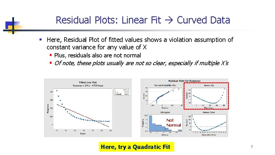
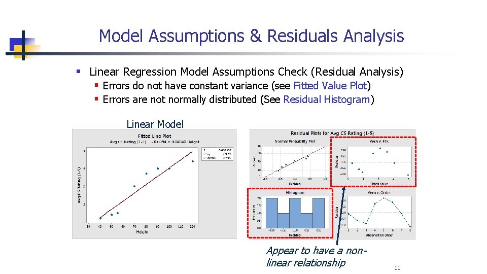
Residual Plots: Linear Fit Curved Data § Here, Residual Plot of fitted values shows a violation assumption of constant variance for any value of X § Plus, residuals also are not normal § Of note, these plots usually are not so clear, especially if multiple X’s Not Normal Here, try a Quadratic Fit 7

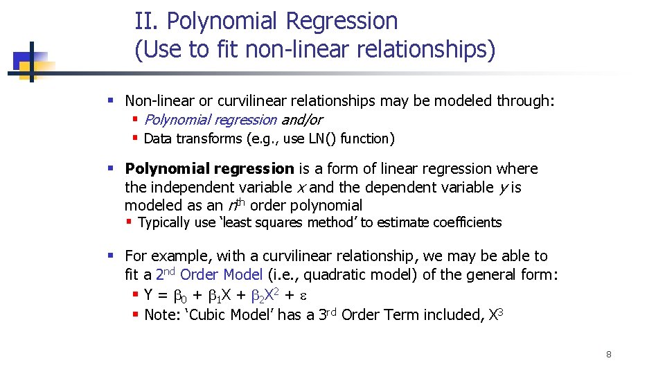
II. Polynomial Regression (Use to fit non-linear relationships) § Non-linear or curvilinear relationships may be modeled through: § Polynomial regression and/or § Data transforms (e. g. , use LN() function) § Polynomial regression is a form of linear regression where the independent variable x and the dependent variable y is modeled as an nth order polynomial § Typically use ‘least squares method’ to estimate coefficients § For example, with a curvilinear relationship, we may be able to fit a 2 nd Order Model (i. e. , quadratic model) of the general form: § Y = b 0 + b 1 X + b 2 X 2 + e § Note: ‘Cubic Model’ has a 3 rd Order Term included, X 3 8

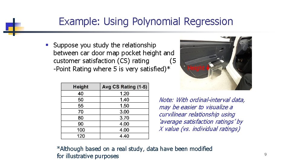
Example: Using Polynomial Regression § Suppose you study the relationship between car door map pocket height and customer satisfaction (CS) rating (5 -Point Rating where 5 is very satisfied)* Height Note: With ordinal-interval data, may be easier to visualize a curvilinear relationship using ‘average satisfaction ratings’ by X value (vs. individual ratings) *Although based on a real study, data have been modified for illustrative purposes 9

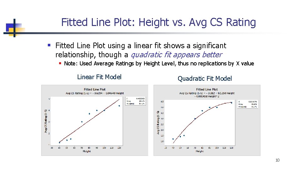
Fitted Line Plot: Height vs. Avg CS Rating § Fitted Line Plot using a linear fit shows a significant relationship, though a quadratic fit appears better § Note: Used Average Ratings by Height Level, thus no replications by X value Linear Fit Model Quadratic Fit Model 10

Model Assumptions & Residuals Analysis § Linear Regression Model Assumptions Check (Residual Analysis) § Errors do not have constant variance (see Fitted Value Plot) § Errors are not normally distributed (See Residual Histogram) Linear Model Appear to have a nonlinear relationship 11

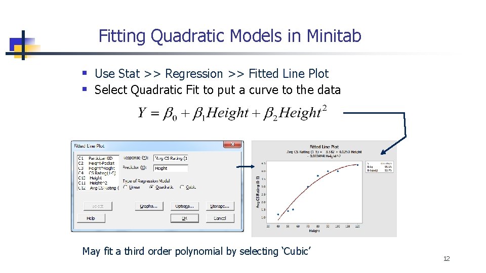
Fitting Quadratic Models in Minitab § Use Stat >> Regression >> Fitted Line Plot § Select Quadratic Fit to put a curve to the data May fit a third order polynomial by selecting ‘Cubic’ 12

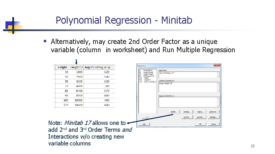
Polynomial Regression - Minitab § Alternatively, may create 2 nd Order Factor as a unique variable (column in worksheet) and Run Multiple Regression Note: Minitab 17 allows one to add 2 nd and 3 rd Order Terms and Interactions w/o creating new variable columns 13

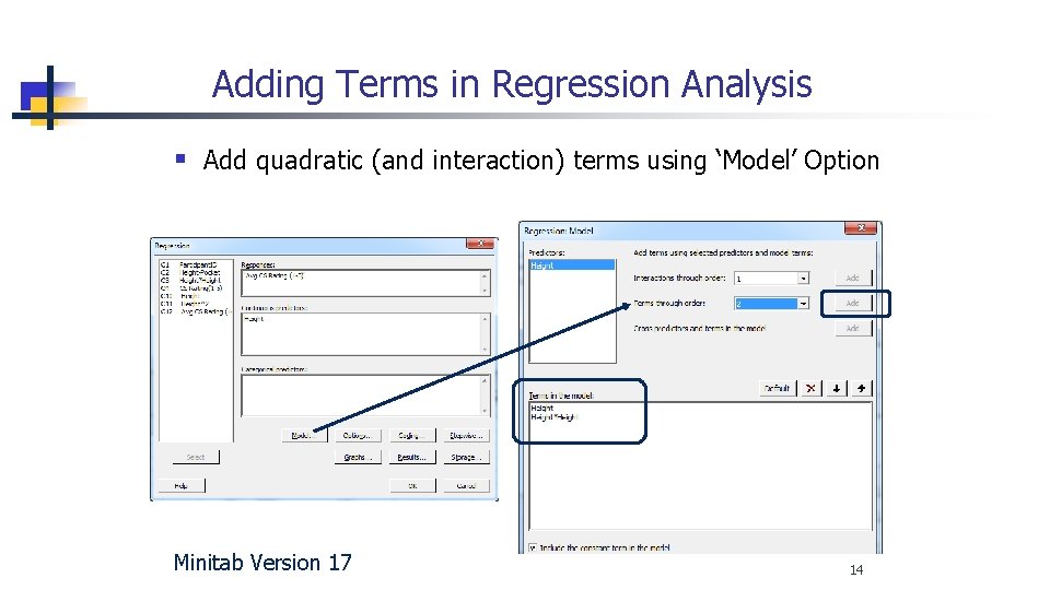
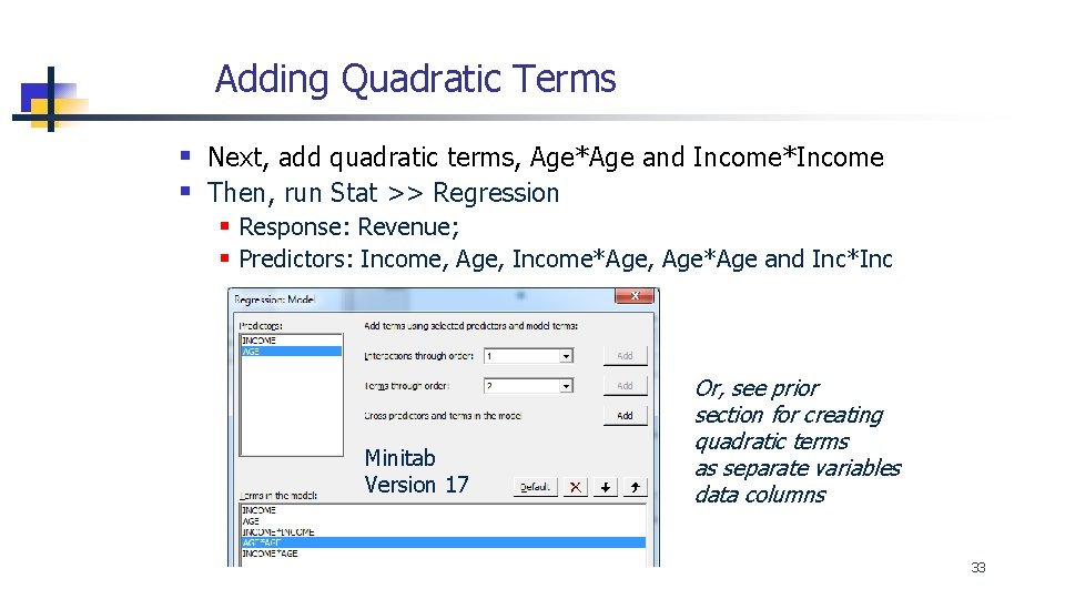
Adding Terms in Regression Analysis § Add quadratic (and interaction) terms using ‘Model’ Option Minitab Version 17 14

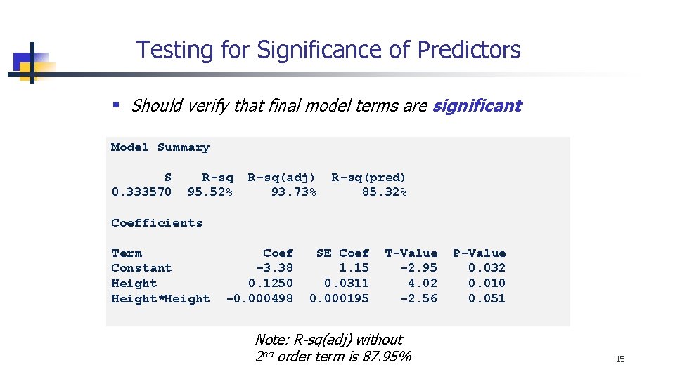
Testing for Significance of Predictors § Should verify that final model terms are significant Model Summary S 0. 333570 R-sq 95. 52% R-sq(adj) 93. 73% R-sq(pred) 85. 32% Coefficients Term Constant Height*Height Coef -3. 38 0. 1250 -0. 000498 SE Coef 1. 15 0. 0311 0. 000195 T-Value -2. 95 4. 02 -2. 56 Note: R-sq(adj) without 2 nd order term is 87. 95% P-Value 0. 032 0. 010 0. 051 15

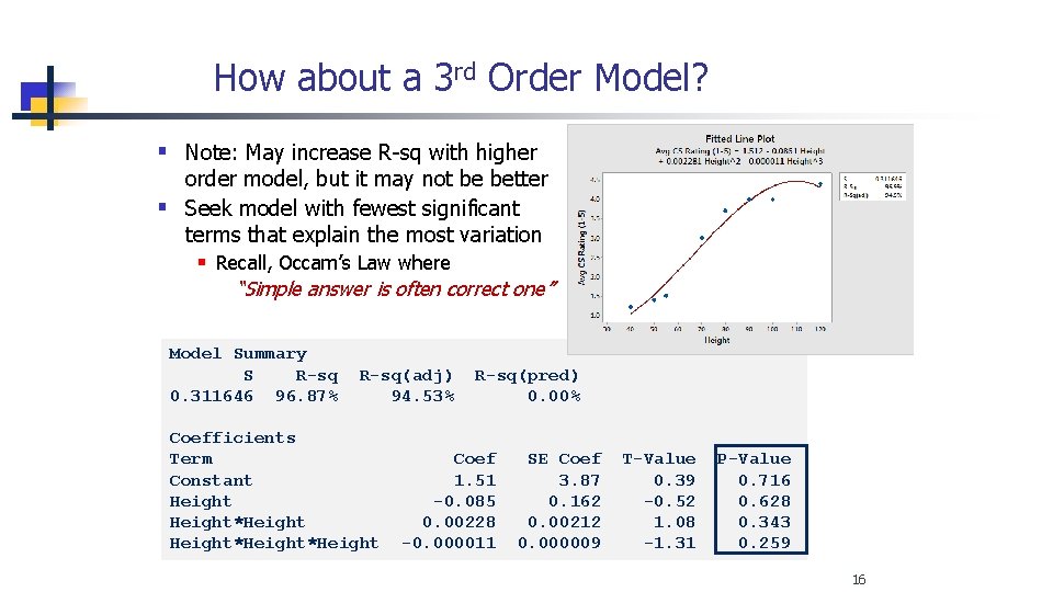
How about a 3 rd Order Model? § Note: May increase R-sq with higher order model, but it may not be better § Seek model with fewest significant terms that explain the most variation § Recall, Occam’s Law where “Simple answer is often correct one” Model Summary S R-sq 0. 311646 96. 87% R-sq(adj) 94. 53% Coefficients Term Constant Height*Height R-sq(pred) 0. 00% Coef 1. 51 -0. 085 0. 00228 -0. 000011 SE Coef 3. 87 0. 162 0. 00212 0. 000009 T-Value 0. 39 -0. 52 1. 08 -1. 31 P-Value 0. 716 0. 628 0. 343 0. 259 16

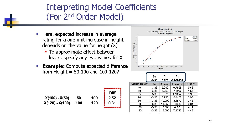
Interpreting Model Coefficients (For 2 nd Order Model) § Here, expected increase in average rating for a one-unit increase in height depends on the value for height (X) § To approximate effect between levels, specify any two values for X § Example: Compute expected difference from Height = 50 -100 and 100 -120? 17

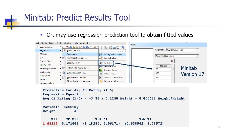
Minitab: Predict Results Tool § Or, may use regression prediction tool to obtain fitted values Minitab Version 17 Prediction for Avg CS Rating (1 -5) Regression Equation Avg CS Rating (1 -5) = -3. 38 + 0. 1250 Height - 0. 000498 Height*Height Variable Height Setting 50 Fit 1. 62214 SE Fit 0. 171002 95% CI (1. 18256, 2. 06171) 95% PI (0. 658562, 2. 58572) 18

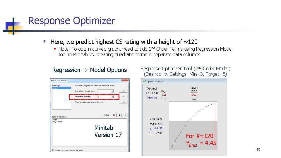
Response Optimizer § Here, we predict highest CS rating with a height of ~120 § Note: To obtain curved graph, need to add 2 nd Order Terms using Regression Model tool in Minitab vs. creating quadratic terms in separate data columns Regression Model Options Minitab Version 17 Response Optimizer Tool (2 nd Order Model) (Desirability Settings: Min=3, Target=5) For X=120 Ypred = 4. 45 19

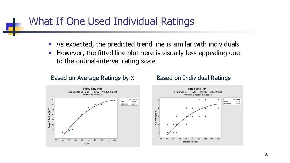
What If One Used Individual Ratings § As expected, the predicted trend line is similar with individuals § However, the fitted line plot here is visually less appealing due to the ordinal-interval rating scale Based on Average Ratings by X Based on Individual Ratings 20

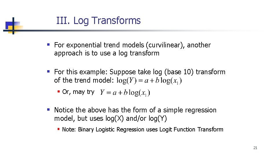
III. Log Transforms § For exponential trend models (curvilinear), another approach is to use a log transform § For this example: Suppose take log (base 10) transform of the trend model: § Or, may try § Notice the above has the form of a simple regression model, but uses log(X) and/or log(Y) § Note: Binary Logistic Regression uses Logit Function Transform 21

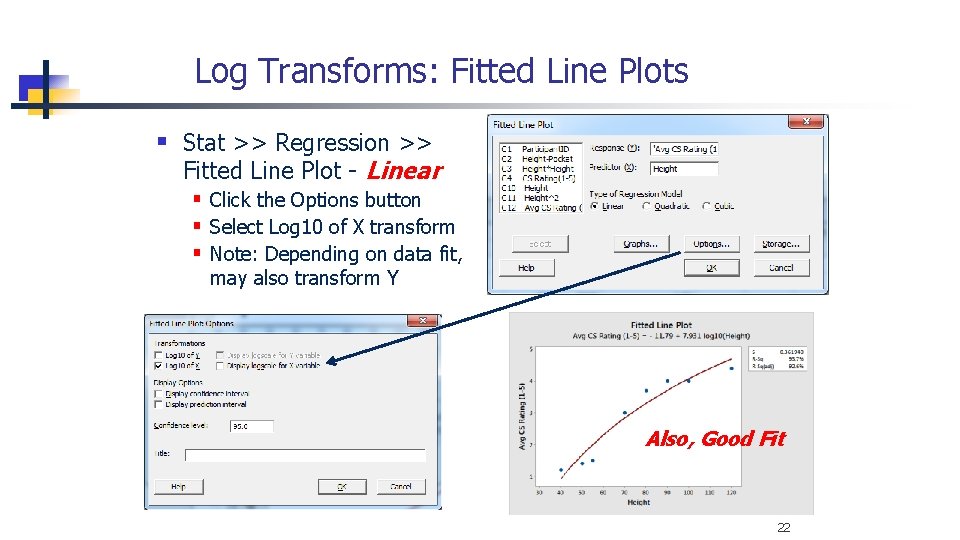
Log Transforms: Fitted Line Plots § Stat >> Regression >> Fitted Line Plot - Linear § Click the Options button § Select Log 10 of X transform § Note: Depending on data fit, may also transform Y Also, Good Fit 22

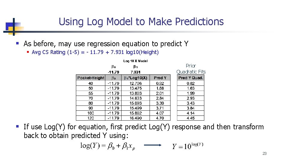
Using Log Model to Make Predictions § As before, may use regression equation to predict Y § Avg CS Rating (1 -5) = - 11. 79 + 7. 931 log 10(Height) Prior Quadratic Fits § If use Log(Y) for equation, first predict Log(Y) response and then transform back to obtain predicted Y using: 23

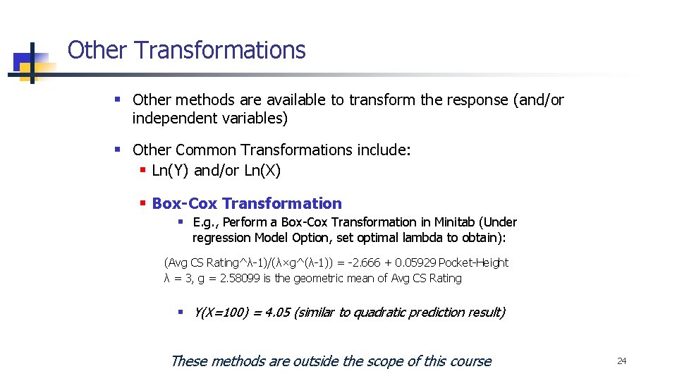
Other Transformations § Other methods are available to transform the response (and/or independent variables) § Other Common Transformations include: § Ln(Y) and/or Ln(X) § Box-Cox Transformation § E. g. , Perform a Box-Cox Transformation in Minitab (Under regression Model Option, set optimal lambda to obtain): (Avg CS Rating^λ-1)/(λ×g^(λ-1)) = -2. 666 + 0. 05929 Pocket-Height λ = 3, g = 2. 58099 is the geometric mean of Avg CS Rating § Y(X=100) = 4. 05 (similar to quadratic prediction result) These methods are outside the scope of this course 24

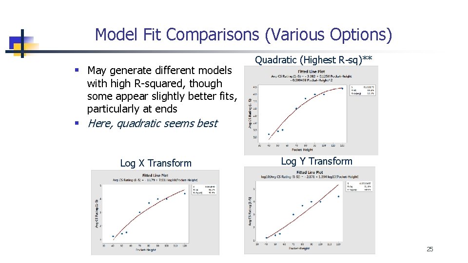
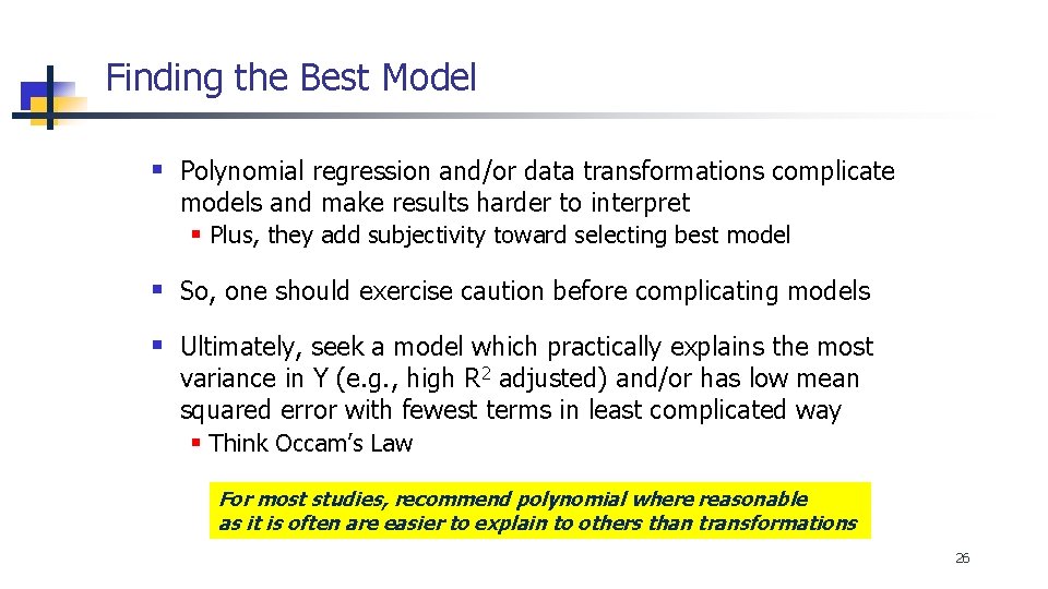
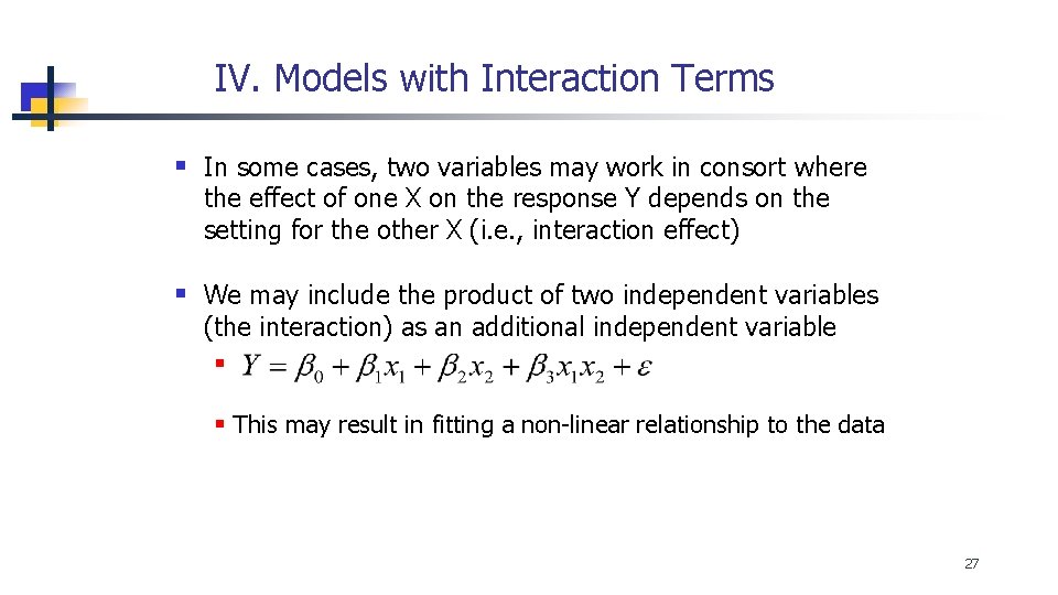
Model Fit Comparisons (Various Options) § May generate different models Quadratic (Highest R-sq)** with high R-squared, though some appear slightly better fits, particularly at ends § Here, quadratic seems best Log X Transform Log Y Transform 25

Finding the Best Model § Polynomial regression and/or data transformations complicate models and make results harder to interpret § Plus, they add subjectivity toward selecting best model § So, one should exercise caution before complicating models § Ultimately, seek a model which practically explains the most variance in Y (e. g. , high R 2 adjusted) and/or has low mean squared error with fewest terms in least complicated way § Think Occam’s Law For most studies, recommend polynomial where reasonable as it is often are easier to explain to others than transformations 26

IV. Models with Interaction Terms § In some cases, two variables may work in consort where the effect of one X on the response Y depends on the setting for the other X (i. e. , interaction effect) § We may include the product of two independent variables (the interaction) as an additional independent variable § § This may result in fitting a non-linear relationship to the data 27

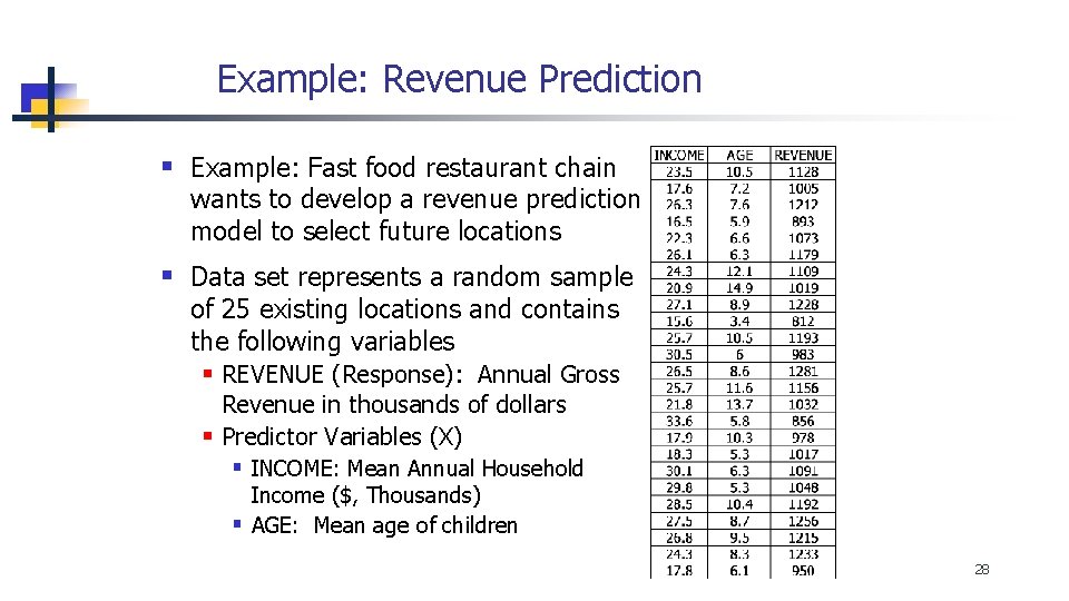
Example: Revenue Prediction § Example: Fast food restaurant chain wants to develop a revenue prediction model to select future locations § Data set represents a random sample of 25 existing locations and contains the following variables § REVENUE (Response): Annual Gross Revenue in thousands of dollars § Predictor Variables (X) § INCOME: Mean Annual Household Income ($, Thousands) § AGE: Mean age of children 28

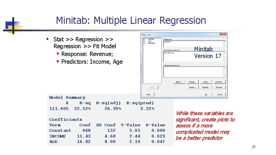
Minitab: Multiple Linear Regression § Stat >> Regression >> Fit Model § Response: Revenue; § Predictors: Income, Age Model Summary S R-sq 111. 605 32. 52% R-sq(adj) 26. 39% Coefficients Term Coef Constant 668 INCOME 11. 43 AGE 16. 82 SE Coef 132 4. 68 8. 00 Minitab Version 17 R-sq(pred) 3. 22% T-Value 5. 05 2. 44 2. 10 P-Value 0. 000 0. 023 0. 047 While these variables are significant, create plots to assess if a more complicated model may be a better predictor 29

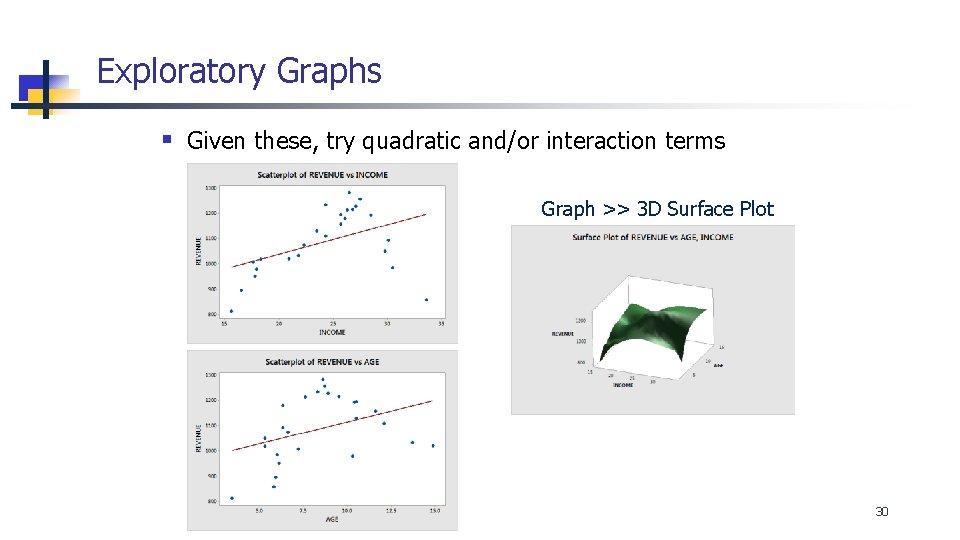
Exploratory Graphs § Given these, try quadratic and/or interaction terms Graph >> 3 D Surface Plot 30

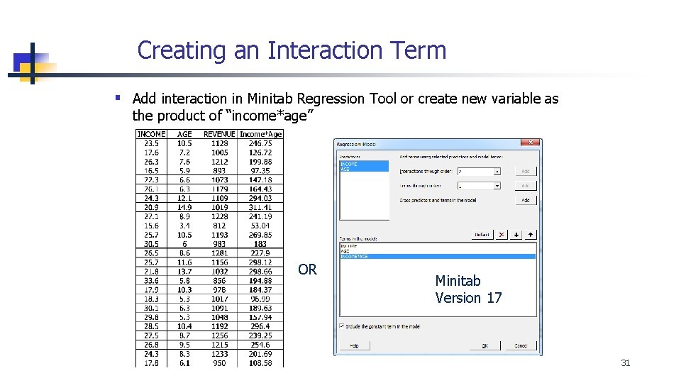
Creating an Interaction Term § Add interaction in Minitab Regression Tool or create new variable as the product of “income*age” OR Minitab Version 17 31

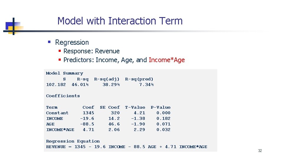
Model with Interaction Term § Regression § Response: Revenue § Predictors: Income, Age, and Income*Age Model Summary S R-sq 102. 182 46. 01% R-sq(adj) 38. 29% R-sq(pred) 7. 34% Coefficients Term Constant INCOME AGE INCOME*AGE Coef 1345 -19. 6 -88. 5 4. 71 SE Coef 320 14. 2 46. 6 2. 06 T-Value 4. 21 -1. 38 -1. 90 2. 29 P-Value 0. 000 0. 182 0. 071 0. 032 Regression Equation REVENUE = 1345 - 19. 6 INCOME - 88. 5 AGE + 4. 71 INCOME*AGE 32

Adding Quadratic Terms § Next, add quadratic terms, Age*Age and Income*Income § Then, run Stat >> Regression § Response: Revenue; § Predictors: Income, Age, Income*Age, Age*Age and Inc*Inc Minitab Version 17 Or, see prior section for creating quadratic terms as separate variables data columns 33

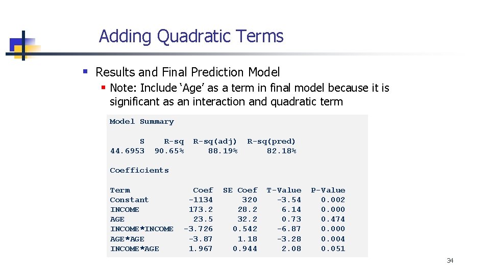
Adding Quadratic Terms § Results and Final Prediction Model § Note: Include ‘Age’ as a term in final model because it is significant as an interaction and quadratic term Model Summary S 44. 6953 R-sq 90. 65% R-sq(adj) 88. 19% R-sq(pred) 82. 18% Coefficients Term Constant INCOME AGE INCOME*INCOME AGE*AGE INCOME*AGE Coef -1134 173. 2 23. 5 -3. 726 -3. 87 1. 967 SE Coef 320 28. 2 32. 2 0. 542 1. 18 0. 944 T-Value -3. 54 6. 14 0. 73 -6. 87 -3. 28 2. 08 P-Value 0. 002 0. 000 0. 474 0. 000 0. 004 0. 051 34

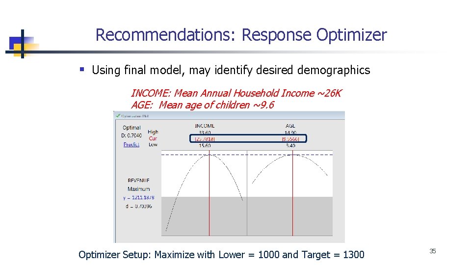
Recommendations: Response Optimizer § Using final model, may identify desired demographics INCOME: Mean Annual Household Income ~26 K AGE: Mean age of children ~9. 6 Optimizer Setup: Maximize with Lower = 1000 and Target = 1300 35

Summary § For non-linear (curvilinear) relationships, may be able to improve model fit using polynomial regression with quadratic/interaction terms and/or data transformations (e. g. , log transforms) § Though this makes it more difficult to interpret factor effects § May include an interaction term if the effect of 1 predictor on the response Y depends on the setting for another predictor 36

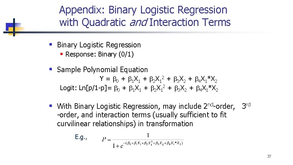
Appendix: Binary Logistic Regression with Quadratic and Interaction Terms § Binary Logistic Regression § Response: Binary (0/1) § Sample Polynomial Equation Y = b 0 + b 1 X 1 + b 2 X 12 + b 3 X 2 + b 4 X 1*X 2 Logit: Ln[p/1 -p]= b 0 + b 1 X 1 + b 2 X 12 + b 3 X 2 + b 4 X 1*X 2 § With Binary Logistic Regression, may include 2 nd-order, 3 rd -order, and interaction terms (usually sufficient to fit curvilinear relationships) in transformation E. g. , 37

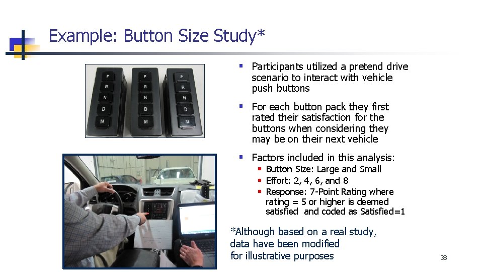
Example: Button Size Study* § Participants utilized a pretend drive scenario to interact with vehicle push buttons § For each button pack they first rated their satisfaction for the buttons when considering they may be on their next vehicle § Factors included in this analysis: § Button Size: Large and Small § Effort: 2, 4, 6, and 8 § Response: 7 -Point Rating where rating = 5 or higher is deemed satisfied and coded as Satisfied=1 *Although based on a real study, data have been modified for illustrative purposes 38

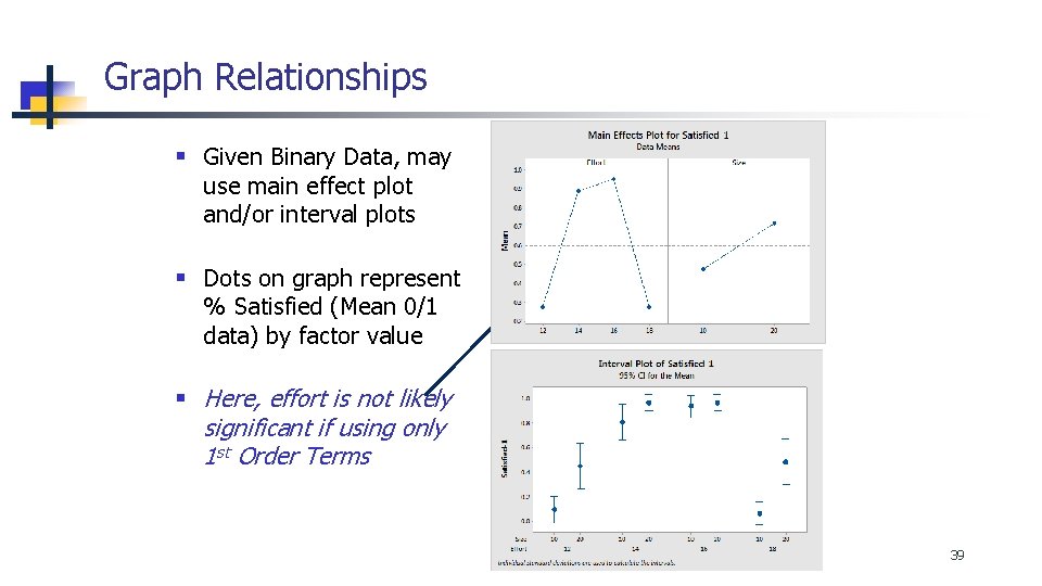
Graph Relationships § Given Binary Data, may use main effect plot and/or interval plots § Dots on graph represent % Satisfied (Mean 0/1 data) by factor value § Here, effort is not likely significant if using only 1 st Order Terms 39

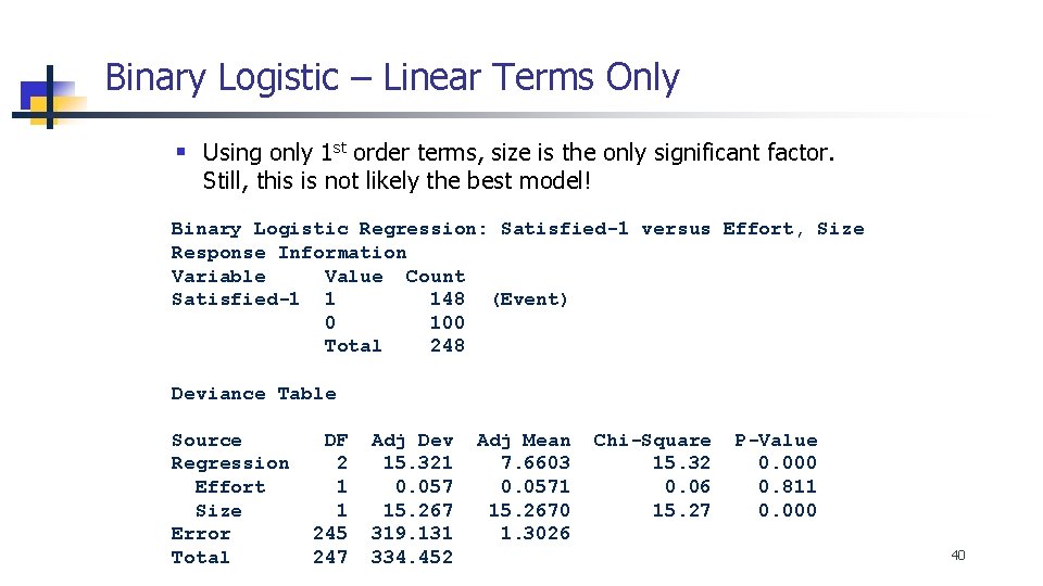
Binary Logistic – Linear Terms Only § Using only 1 st order terms, size is the only significant factor. Still, this is not likely the best model! Binary Logistic Regression: Satisfied-1 versus Effort, Size Response Information Variable Value Count Satisfied-1 1 148 (Event) 0 100 Total 248 Deviance Table Source Regression Effort Size Error Total DF 2 1 1 245 247 Adj Dev 15. 321 0. 057 15. 267 319. 131 334. 452 Adj Mean 7. 6603 0. 0571 15. 2670 1. 3026 Chi-Square 15. 32 0. 06 15. 27 P-Value 0. 000 0. 811 0. 000 40

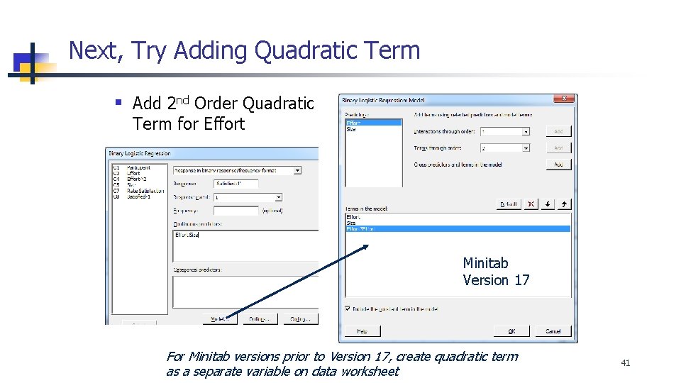
Next, Try Adding Quadratic Term § Add 2 nd Order Quadratic Term for Effort Minitab Version 17 For Minitab versions prior to Version 17, create quadratic term as a separate variable on data worksheet 41

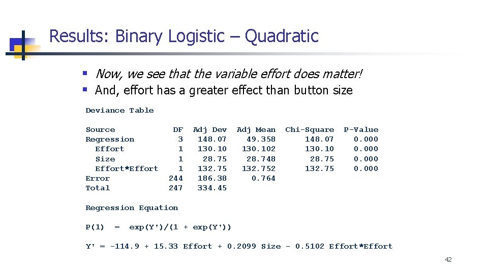
Results: Binary Logistic – Quadratic § Now, we see that the variable effort does matter! § And, effort has a greater effect than button size Deviance Table Source Regression Effort Size Effort*Effort Error Total DF 3 1 1 1 244 247 Adj Dev 148. 07 130. 10 28. 75 132. 75 186. 38 334. 45 Adj Mean 49. 358 130. 102 28. 748 132. 752 0. 764 Chi-Square 148. 07 130. 10 28. 75 132. 75 P-Value 0. 000 Regression Equation P(1) = exp(Y')/(1 + exp(Y')) Y' = -114. 9 + 15. 33 Effort + 0. 2099 Size - 0. 5102 Effort*Effort 42

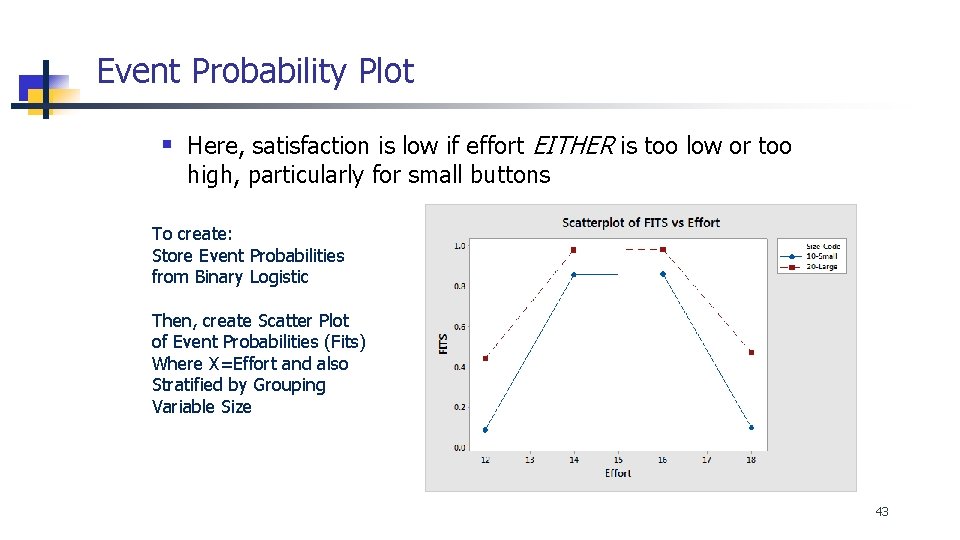
Event Probability Plot § Here, satisfaction is low if effort EITHER is too low or too high, particularly for small buttons To create: Store Event Probabilities from Binary Logistic Then, create Scatter Plot of Event Probabilities (Fits) Where X=Effort and also Stratified by Grouping Variable Size 43

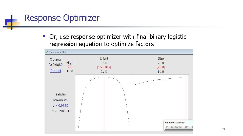
Response Optimizer § Or, use response optimizer with final binary logistic regression equation to optimize factors 44