Complex Numbers By default MATLAB treats all numbers

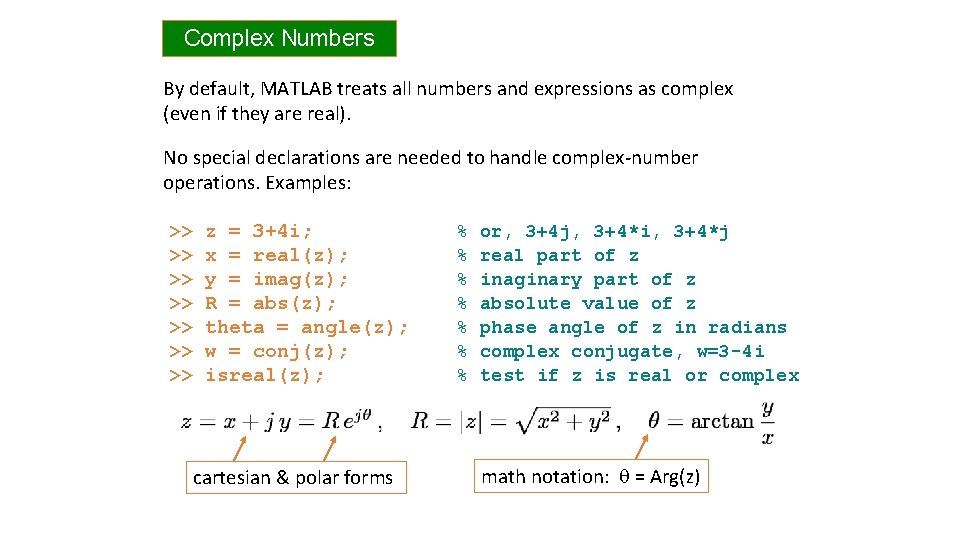
Complex Numbers By default, MATLAB treats all numbers and expressions as complex (even if they are real). No special declarations are needed to handle complex-number operations. Examples: >> >> z = 3+4 i; x = real(z); y = imag(z); R = abs(z); theta = angle(z); w = conj(z); isreal(z); cartesian & polar forms % % % % or, 3+4 j, 3+4*i, 3+4*j real part of z inaginary part of z absolute value of z phase angle of z in radians complex conjugate, w=3 -4 i test if z is real or complex math notation: q = Arg(z)

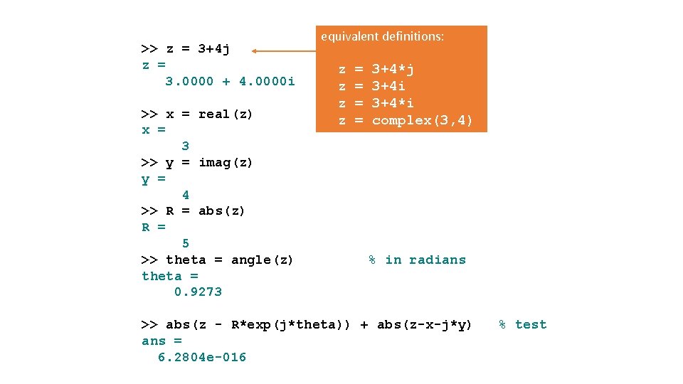
>> z = 3+4 j z = 3. 0000 + 4. 0000 i >> x = real(z) x = 3 >> y = imag(z) y = 4 >> R = abs(z) R = 5 >> theta = angle(z) theta = 0. 9273 equivalent definitions: z z = = 3+4*j 3+4 i 3+4*i complex(3, 4) % in radians >> abs(z - R*exp(j*theta)) + abs(z-x-j*y) ans = 6. 2804 e-016 % test

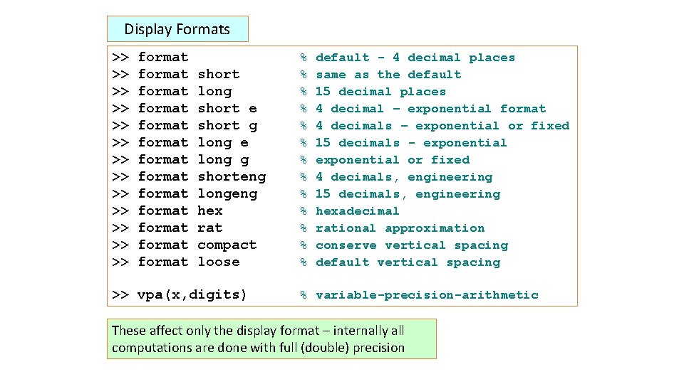
Display Formats >> >> >> >> format format format format short long short e short g long e long g shorteng longeng hex rat compact loose >> vpa(x, digits) % % % % default - 4 decimal places same as the default 15 decimal places 4 decimal – exponential format 4 decimals – exponential or fixed 15 decimals - exponential or fixed 4 decimals, engineering 15 decimals, engineering hexadecimal rational approximation conserve vertical spacing default vertical spacing % variable-precision-arithmetic These affect only the display format – internally all computations are done with full (double) precision

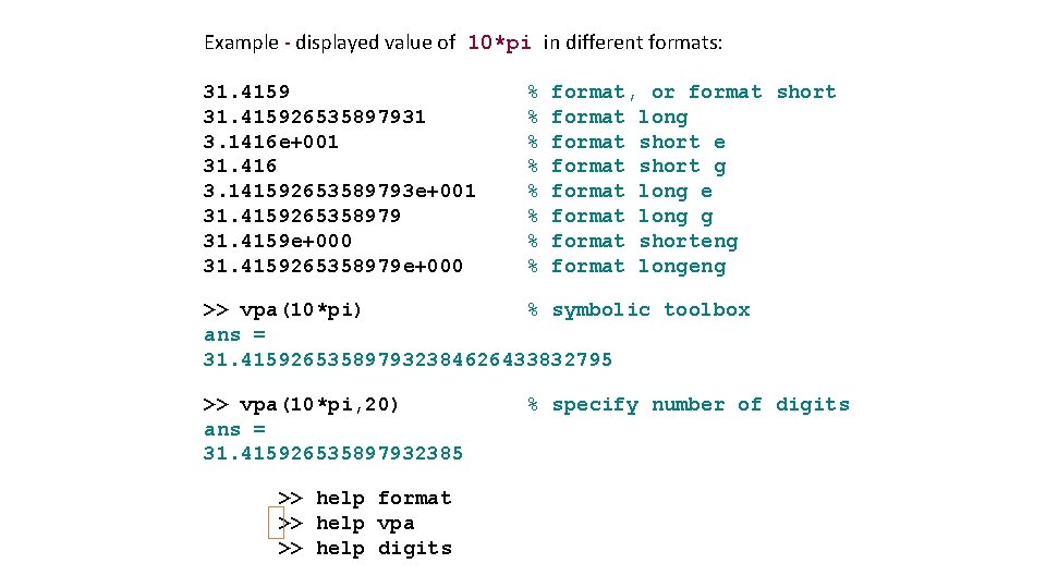
Example - displayed value of 10*pi in different formats: 31. 415926535897931 3. 1416 e+001 31. 416 3. 141592653589793 e+001 31. 4159265358979 31. 4159 e+000 31. 4159265358979 e+000 % % % % format, or format short format long format short e format short g format long e format long g format shorteng format longeng >> vpa(10*pi) % symbolic toolbox ans = 31. 415926535897932384626433832795 >> vpa(10*pi, 20) ans = 31. 415926535897932385 >> help format >> help vpa >> help digits % specify number of digits

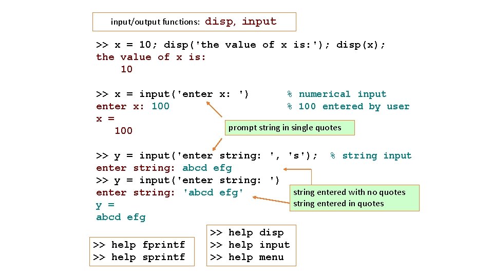
input/output functions: disp, input >> x = 10; disp('the value of x is: '); disp(x); the value of x is: 10 >> x = input('enter x: ') % numerical input enter x: 100 % 100 entered by user x = prompt string in single quotes 100 >> y = input('enter string: ', 's'); % string input enter string: abcd efg >> y = input('enter string: ') string entered with no quotes enter string: 'abcd efg' string entered in quotes y = abcd efg >> help disp >> help fprintf >> help input >> help sprintf >> help menu

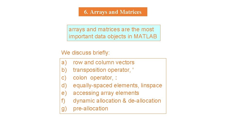
6. Arrays and Matrices arrays and matrices are the most important data objects in MATLAB We discuss briefly: a) b) c) d) e) f) g) row and column vectors transposition operator, ' colon operator, : equally-spaced elements, linspace accessing array elements dynamic allocation & de-allocation pre-allocation

Compare the two alternative computations: x = [2, -3, 4, 1, 5, 8]; y = zeros(size(x)); for n = 1: length(x) y(n) = x(n)^2; end x = [2, -3, 4, 1, 5, 8]; y = x. ^2; element-wise exponentiation ordinary exponentiation ^ answer: y = [4, 9, 16, 1, 25, 64] . ^

>> x = [0 1 2 3 4 5] x = 0 1 2 >> x = 0: 5 x = 0 1 % row vector 3 4 5 % row vector 2 3 4 5 >> x = [0 1 2 3 4 5]' % column vector, (0: 5)' x = 0 the prime operator, ', or transpose, turns row 1 vectors into column vectors, and vice versa 2 3 caveat: ' is actually conjugate transpose, 4 use dot-prime, . ' , for transpose w/o conjugation 5

>> z = [i; 1+2 i; 1 -i] z = 0 + 1. 0000 i 1. 0000 + 2. 0000 i 1. 0000 - 1. 0000 i >> z. ' ans = % transpose without conjugation 0 + 1. 0000 i >> z' ans = % column vector 1. 0000 + 2. 0000 i 1. 0000 - 1. 0000 i % transpose with conjugation 0 - 1. 0000 i 1. 0000 - 2. 0000 i 1. 0000 + 1. 0000 i >> (z. ')' % same as (z'). ' , or, conj(z) ans = 0 - 1. 0000 i 1. 0000 - 2. 0000 i 1. 0000 + 1. 0000 i

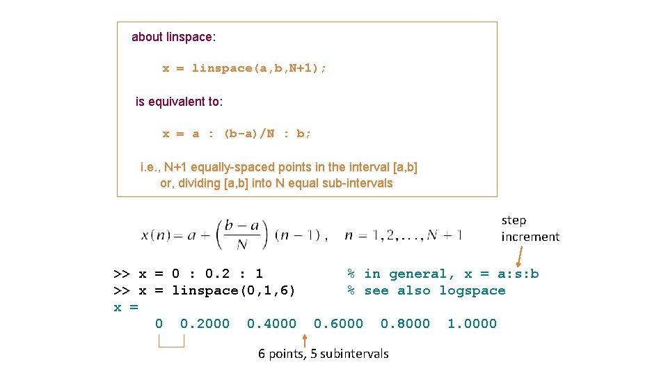
about linspace: x = linspace(a, b, N+1); is equivalent to: x = a : (b-a)/N : b; i. e. , N+1 equally-spaced points in the interval [a, b] or, dividing [a, b] into N equal sub-intervals step increment >> x = 0 : 0. 2 : 1 >> x = linspace(0, 1, 6) x = 0 0. 2000 0. 4000 % in general, x = a: s: b % see also logspace 0. 6000 0. 8000 6 points, 5 subintervals 1. 0000

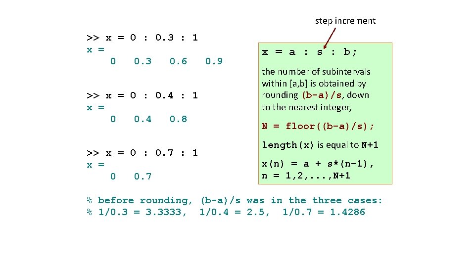
step increment >> x = 0 : 0. 3 : 1 x = 0 0. 3 0. 6 0. 9 >> x = 0 : 0. 4 : 1 x = 0 0. 4 0. 8 >> x = 0 : 0. 7 : 1 x = 0 0. 7 x = a : s : b; the number of subintervals within [a, b] is obtained by rounding (b-a)/s, down to the nearest integer, N = floor((b-a)/s); length(x) is equal to N+1 x(n) = a + s*(n-1), n = 1, 2, . . . , N+1 % before rounding, (b-a)/s was in the three cases: % 1/0. 3 = 3. 3333, 1/0. 4 = 2. 5, 1/0. 7 = 1. 4286

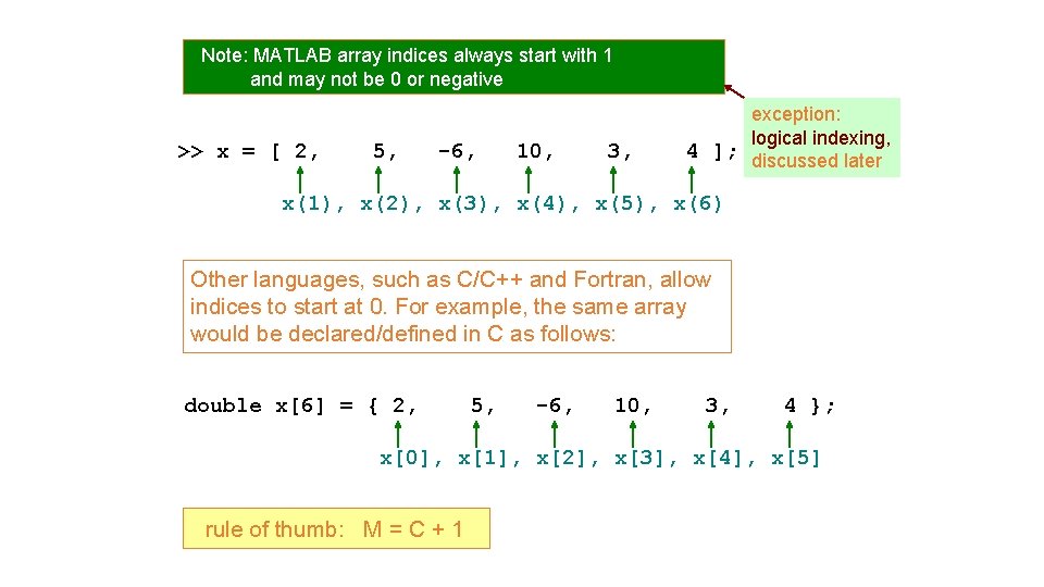
Note: MATLAB array indices always start with 1 and may not be 0 or negative >> x = [ 2, 5, -6, 10, 3, exception: logical indexing, 4 ]; discussed later x(1), x(2), x(3), x(4), x(5), x(6) Other languages, such as C/C++ and Fortran, allow indices to start at 0. For example, the same array would be declared/defined in C as follows: double x[6] = { 2, 5, -6, 10, 3, 4 }; x[0], x[1], x[2], x[3], x[4], x[5] rule of thumb: M = C + 1

accessing array entries: >> x = [2, 5, -6, 10, 3, 4] x = 2 5 -6 10 3 4 >> length(x) ans = 6 % length of x, see also size(x) >> x(1) ans = 2 % first entry >> x(3) ans = -6 % third entry >> x(end) ans = 4 % last entry – need not know length

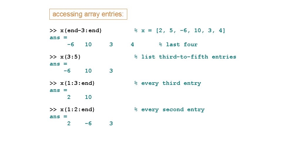
accessing array entries: >> x(end-3: end) ans = -6 10 >> x(3: 5) ans = -6 10 % x = [2, 5, -6, 10, 3, 4] 3 4 % last four % list third-to-fifth entries 3 >> x(1: 3: end) ans = 2 10 % every third entry >> x(1: 2: end) ans = 2 -6 % every second entry 3

accessing array entries: >> x = [2, 5, -6, 10, 3, 4]; >> x(end: -1: 1) ans = 4 3 10 >> x([3, 1, 5]) ans = -6 2 >> x(end+3) = 8 x = 2 5 -6 % list backwards, same as fliplr(x) -6 5 2 % list [x(3), x(1), x(5)] 3 10 3 4 0 automatic memory re-allocation 0 8

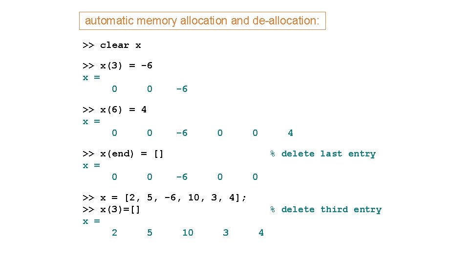
automatic memory allocation and de-allocation: >> clear x >> x(3) = -6 x = 0 0 -6 >> x(6) = 4 x = 0 0 -6 >> x(end) = [] x = 0 0 4 % delete last entry -6 0 >> x = [2, 5, -6, 10, 3, 4]; >> x(3)=[] x = 2 5 10 3 0 % delete third entry 4

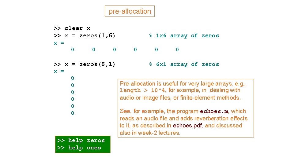
pre-allocation >> clear x >> x = zeros(1, 6) % 1 x 6 array of zeros x = 0 0 0 >> x = zeros(6, 1) 0 0 0 % 6 x 1 array of zeros x = 0 0 0 >> help zeros >> help ones Pre-allocation is useful for very large arrays, e. g. , length > 10^4, for example, in dealing with audio or image files, or finite-element methods. See, for example, the program echoes. m, which reads an audio file and adds reverberation effects to it, as described in echoes. pdf, and discussed also in week-2 lectures.

illustrating dynamic allocation & pre-allocation clear x; for k=[3, 7, 10] x(k) = 3 + 0. 1*k; disp(x); end 0. 0 0. 0 3. 3 0. 0 x = zeros(1, 10); for k=[3, 7, 10] x(k) = 3 + 0. 1*k; disp(x); end 0. 0 0. 0 3. 3 0. 0 % k runs successively through % the values of [3, 7, 10] % diplay current vector x 0. 0 3. 7 0. 0 4. 0 % pre-allocate x to length 10 0. 0 3. 7 0. 0 0. 0 4. 0