COMPILERS Liveness Analysis hussein suleman uct csc 3003

COMPILERS Liveness Analysis hussein suleman uct csc 3003 s 2007

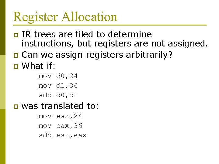
Register Allocation IR trees are tiled to determine instructions, but registers are not assigned. p Can we assign registers arbitrarily? p What if: p mov d 0, 24 mov d 1, 36 add d 0, d 1 p was translated to: mov eax, 24 mov eax, 36 add eax, eax

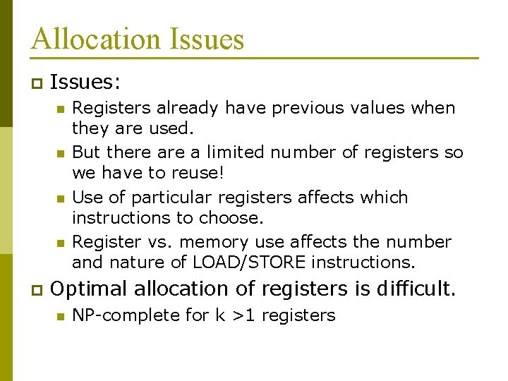
Allocation Issues p Issues: n n p Registers already have previous values when they are used. But there a limited number of registers so we have to reuse! Use of particular registers affects which instructions to choose. Register vs. memory use affects the number and nature of LOAD/STORE instructions. Optimal allocation of registers is difficult. n NP-complete for k >1 registers

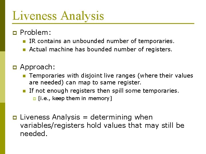
Liveness Analysis p Problem: n n p IR contains an unbounded number of temporaries. Actual machine has bounded number of registers. Approach: n n Temporaries with disjoint live ranges (where their values are needed) can map to same register. If not enough registers then spill some temporaries. p p [i. e. , keep them in memory] Liveness Analysis = determining when variables/registers hold values that may still be needed.

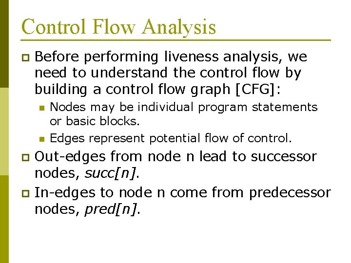
Control Flow Analysis p Before performing liveness analysis, we need to understand the control flow by building a control flow graph [CFG]: n n Nodes may be individual program statements or basic blocks. Edges represent potential flow of control. Out-edges from node n lead to successor nodes, succ[n]. p In-edges to node n come from predecessor nodes, pred[n]. p

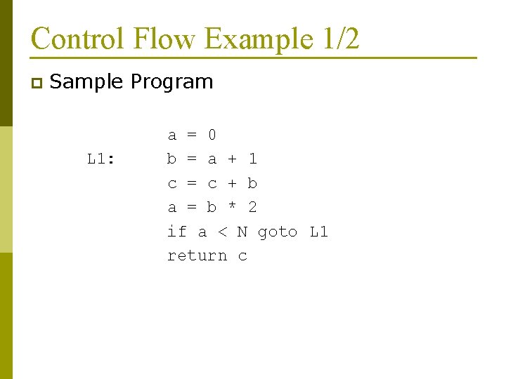
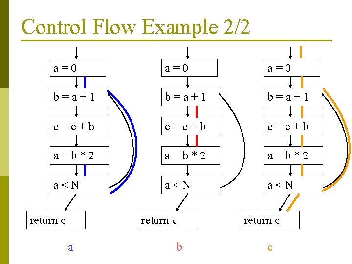
Control Flow Example 1/2 p Sample Program L 1: a = 0 b = a + 1 c = c + b a = b * 2 if a < N goto L 1 return c

Control Flow Example 2/2 a=0 a=0 b=a+1 c=c+b a=b*2 a<N a<N return c a b return c c

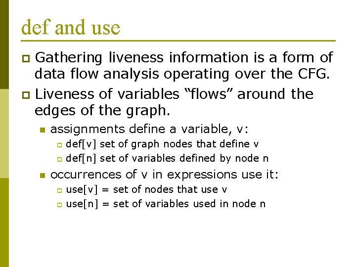
def and use Gathering liveness information is a form of data flow analysis operating over the CFG. p Liveness of variables “flows” around the edges of the graph. p n assignments define a variable, v: def[v] set of graph nodes that define v p def[n] set of variables defined by node n p n occurrences of v in expressions use it: use[v] = set of nodes that use v p use[n] = set of variables used in node n p

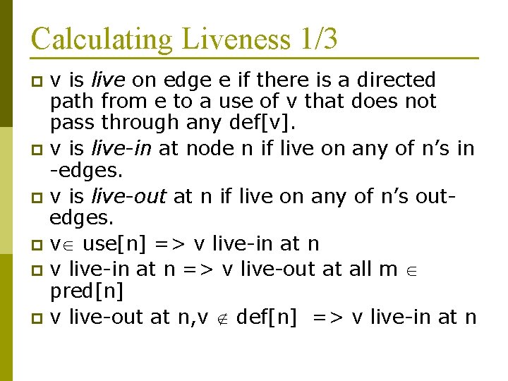
Calculating Liveness 1/3 v is live on edge e if there is a directed path from e to a use of v that does not pass through any def[v]. p v is live-in at node n if live on any of n’s in -edges. p v is live-out at n if live on any of n’s outedges. p v use[n] => v live-in at n p v live-in at n => v live-out at all m pred[n] p v live-out at n, v def[n] => v live-in at n p

Calculating Liveness 2/3 p Define: n n p in[n]: variables live-in at n out[n]: variables live-out at n Then: n n n out[n] = in[s] s succ[n] for a single node successor, p succ[n] = {} => out[n] = {}

Calculating Liveness 3/3 p Note: n n in[n] use[n] in[n] out[n] - def[n] use[n] and def[n] are constant [independent of control flow] p Now, p v in[n] iff v use[n] or v out[n] def[n] p Thus, in[n] = use[n] [out[n] - def[n]] p

Iterative Liveness Calculation Algorithm foreach n {in[n] = {}; out[n] = {}} repeat foreach n in’[n] = in[n]; out’[n] = out[n]; in[n] = use[n] (out[n] - def[n]) out[n] = in[s] s succ[n] until n (in’[n] = in[n]) & (out’[n] = out[n])

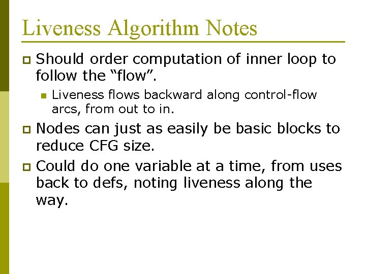
Liveness Algorithm Notes p Should order computation of inner loop to follow the “flow”. n Liveness flows backward along control-flow arcs, from out to in. Nodes can just as easily be basic blocks to reduce CFG size. p Could do one variable at a time, from uses back to defs, noting liveness along the way. p

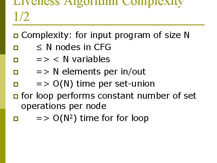
Liveness Algorithm Complexity 1/2 Complexity: for input program of size N p ≤ N nodes in CFG p => < N variables p => N elements per in/out p => O(N) time per set-union p for loop performs constant number of set operations per node p => O(N 2) time for loop p

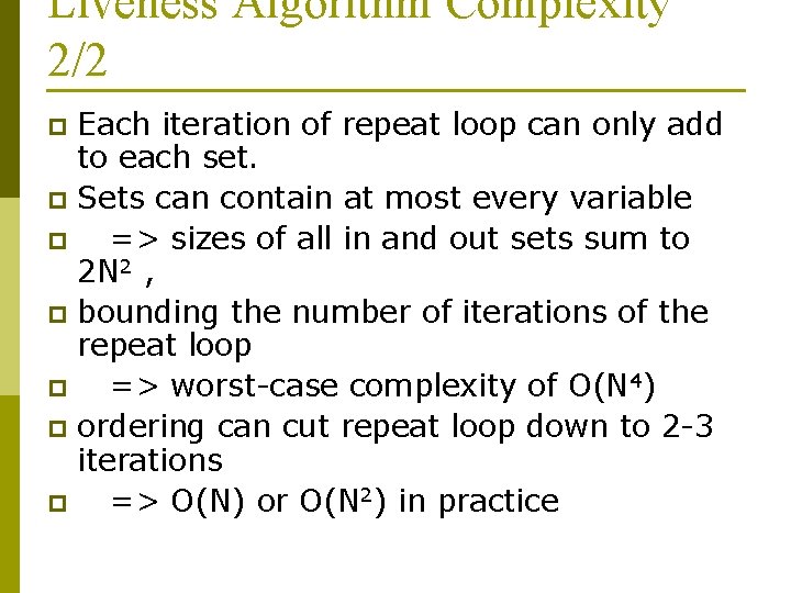
Liveness Algorithm Complexity 2/2 Each iteration of repeat loop can only add to each set. p Sets can contain at most every variable p => sizes of all in and out sets sum to 2 N 2 , p bounding the number of iterations of the repeat loop p => worst-case complexity of O(N 4) p ordering can cut repeat loop down to 2 -3 iterations p => O(N) or O(N 2) in practice p

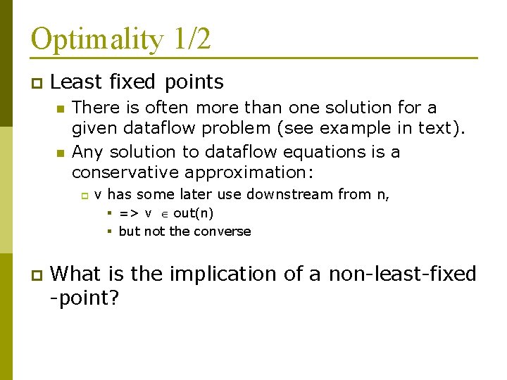
Optimality 1/2 p Least fixed points n n There is often more than one solution for a given dataflow problem (see example in text). Any solution to dataflow equations is a conservative approximation: p v has some later use downstream from n, § => v out(n) § but not the converse p What is the implication of a non-least-fixed -point?

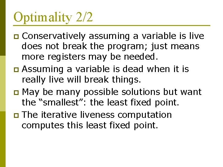
Optimality 2/2 Conservatively assuming a variable is live does not break the program; just means more registers may be needed. p Assuming a variable is dead when it is really live will break things. p May be many possible solutions but want the “smallest”: the least fixed point. p The iterative liveness computation computes this least fixed point. p