Comparison of different Bayesian spatiotemporal models using R

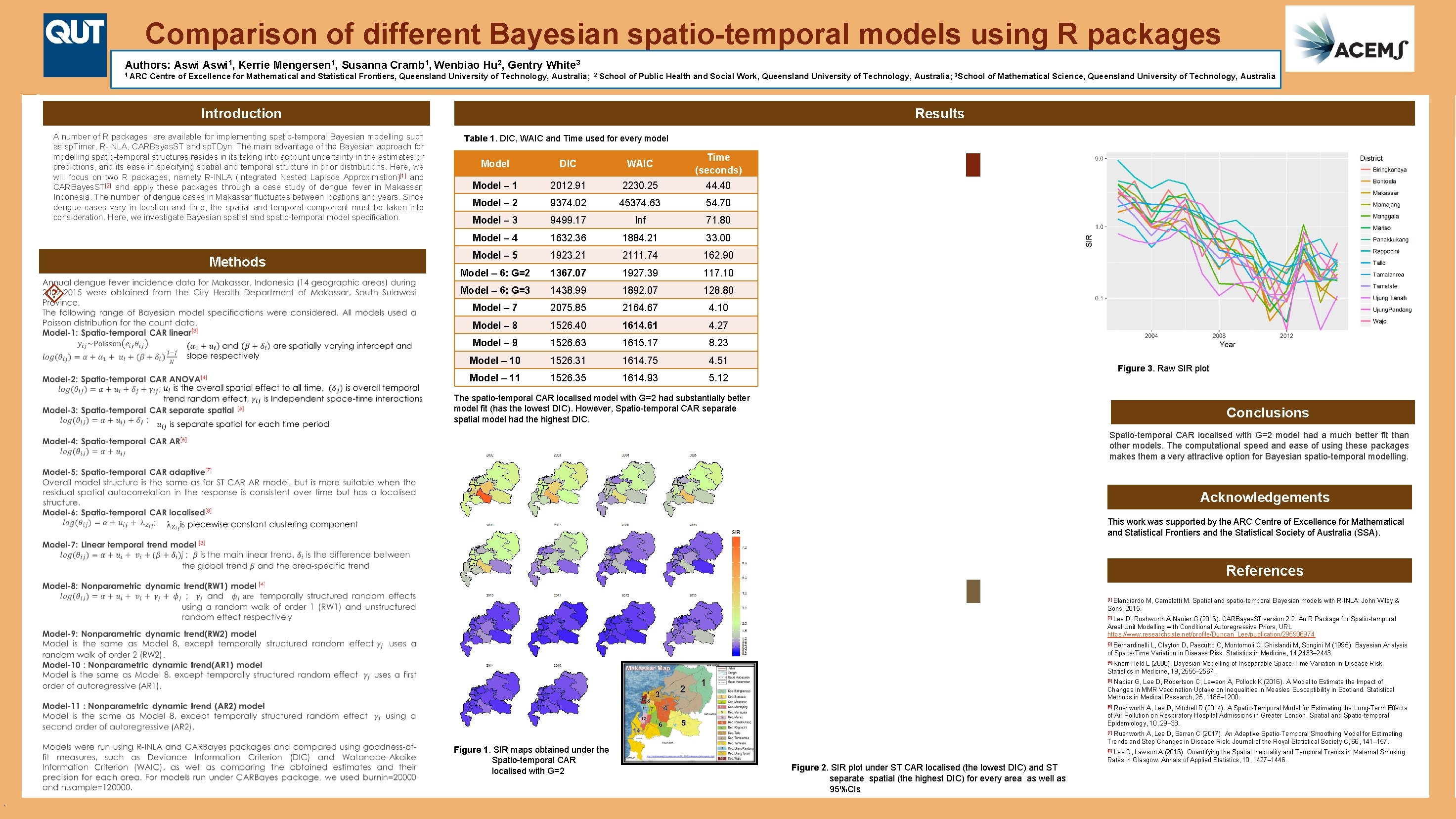
Comparison of different Bayesian spatio-temporal models using R packages Authors: Aswi 1, Kerrie Mengersen 1, Susanna Cramb 1, Wenbiao Hu 2, Gentry White 3 1 ARC Centre of Excellence for Mathematical and Statistical Frontiers, Queensland University of Technology, Australia; 2 School of Public Health and Social Work, Queensland University of Technology, Australia; 3 School of Mathematical Science, Queensland University of Technology, Australia Results Introduction A number of R packages are available for implementing spatio-temporal Bayesian modelling such as sp. Timer, R-INLA, CARBayes. ST and sp. TDyn. The main advantage of the Bayesian approach for modelling spatio-temporal structures resides in its taking into account uncertainty in the estimates or predictions, and its ease in specifying spatial and temporal structure in prior distributions. Here, we will focus on two R packages, namely R-INLA (Integrated Nested Laplace Approximation)[1] and CARBayes. ST[2] and apply these packages through a case study of dengue fever in Makassar, Indonesia. The number of dengue cases in Makassar fluctuates between locations and years. Since dengue cases vary in location and time, the spatial and temporal component must be taken into consideration. Here, we investigate Bayesian spatial and spatio-temporal model specification. Methods Table 1. DIC, WAIC and Time used for every model Model DIC WAIC Time (seconds) Model – 1 2012. 91 2230. 25 44. 40 Model – 2 9374. 02 45374. 63 54. 70 Model – 3 9499. 17 Inf 71. 80 Model – 4 1632. 36 1884. 21 33. 00 Model – 5 1923. 21 2111. 74 162. 90 Model – 6: G=2 1367. 07 1927. 39 117. 10 Model – 6: G=3 1438. 99 1892. 07 128. 80 Model – 7 2075. 85 2164. 67 4. 10 Model – 8 1526. 40 1614. 61 4. 27 Model – 9 1526. 63 1615. 17 8. 23 Model – 10 1526. 31 1614. 75 4. 51 Model – 11 1526. 35 1614. 93 5. 12 Figure 3. Raw SIR plot The spatio-temporal CAR localised model with G=2 had substantially better model fit (has the lowest DIC). However, Spatio-temporal CAR separate spatial model had the highest DIC. Conclusions Spatio-temporal CAR localised with G=2 model had a much better fit than other models. The computational speed and ease of using these packages makes them a very attractive option for Bayesian spatio-temporal modelling. Acknowledgements This work was supported by the ARC Centre of Excellence for Mathematical and Statistical Frontiers and the Statistical Society of Australia (SSA). References [1] Blangiardo M, Cameletti M. Spatial and spatio-temporal Bayesian models with R-INLA: John Wiley & Sons; 2015. [2] Lee D, Rushworth A, Naoier G (2016). CARBayes. ST version 2. 2: An R Package for Spatio-temporal Areal Unit Modelling with Conditional Autoregressive Priors, URL https: //www. researchgate. net/profile/Duncan_Lee/publication/295906974 [3] Bernardinelli L, Clayton D, Pascutto C, Montomoli C, Ghislandi M, Songini M (1995). Bayesian Analysis of Space-Time Variation in Disease Risk. Statistics in Medicine, 14, 2433– 2443. [4] Knorr-Held L (2000). Bayesian Modelling of Inseparable Space-Time Variation in Disease Risk. Statistics in Medicine, 19, 2555– 2567. Napier G, Lee D, Robertson C, Lawson A, Pollock K (2016). A Model to Estimate the Impact of Changes in MMR Vaccination Uptake on Inequalities in Measles Susceptibility in Scotland. Statistical Methods in Medical Research, 25, 1185– 1200. [5] Rushworth A, Lee D, Mitchell R (2014). A Spatio-Temporal Model for Estimating the Long-Term Effects of Air Pollution on Respiratory Hospital Admissions in Greater London. Spatial and Spatio-temporal Epidemiology, 10, 29– 38. [6] Rushworth A, Lee D, Sarran C (2017). An Adaptive Spatio-Temporal Smoothing Model for Estimating Trends and Step Changes in Disease Risk. Journal of the Royal Statistical Society C, 66, 141– 157. [7] Figure 1. SIR maps obtained under the Spatio-temporal CAR localised with G=2 ` Lee D, Lawson A (2016). Quantifying the Spatial Inequality and Temporal Trends in Maternal Smoking Rates in Glasgow. Annals of Applied Statistics, 10, 1427– 1446. [8] Figure 2. SIR plot under ST CAR localised (the lowest DIC) and ST separate spatial (the highest DIC) for every area as well as 95%CIs