Comparing Regression Lines From Independent Samples The Design

Comparing Regression Lines From Independent Samples

The Design • • • You have two or more groups. One or more continuous predictors (C). And one continuous outcome variable (Y). You want to know if Y = a + b 1 C 1 + … + bp. Cp + error Is the same across groups.

Poteat, Wuensch, & Gregg • Predictive validity study • Children referred for school psychology services • Does Grades = a + b IQ + error • Differ across races? • Called a “Potthoff analysis” by school psychologists • Differences fell short of significance.

Two Groups, One X • Y = a + b 1 C + b 2 G + b 3 C G • If there are more than two groups, groups is represented by k-1 dummy variables • Wuensch, Jenkins, & Poteat • Y = Attitude to animals • C = Misanthropy • G = High idealism or not

SAS • • • Potthoff. sas -- download Potthoff. dat – download Point program file to data file Run the program Data step: Mx. I = Misanth Idealism Page 1: Ignoring idealism, is a. 2 corr between misanthropy and attitude to animals.

Zero-Order Correlations

Interpretation • Misanthropy is significantly related to support for animal rights. • The two idealism groups do not differ significantly on support for animal rights – rpb =. 092. • The two idealism groups do not differ significantly on misanthropy – rpb = -. 099.

Four Regression Models • • • Proc Reg; CGI: model ar = misanth idealism Mx. I; C: model ar=misanth; CG: model ar = misanth idealism; CI: model ar = misanth Mx. I;

Model CGI Analysis of Variance Source DF Sum of Squares Model 3 4. 05237 Error 150 Corrected 153 Total Mean Square 1. 35079 39. 73945 0. 26493 43. 79182 F Value Pr > F 5. 10 0. 0022

Model C Analysis of Variance Source DF Sum of Squares Model 1 2. 13252 Error 152 41. 65930 Corrected 153 43. 79182 Total Mean Square 2. 13252 0. 27407 F Value Pr > F 7. 78 0. 0060

Test of Coincidence • Compare model CGI with model C • Use a partial F test p =. 029

Conclusion • This was a simultaneous test of intercept and slopes. • We conclude that the two groups differ with respect to • The intercepts, or • The slopes, • Or both.

An Easier Way proc reg; model ar = misanth idealism Mx. I; TEST idealism=0, Mx. I=0; run; Test 1 Results for Dependent Variable ar Source Numerator Denominator DF Mean Square 2 0. 95992 150 0. 26493 F Value Pr > F 3. 62 0. 0291

Model CI Analysis of Variance Source DF Sum of Squares Model 2 2. 29525 Error 151 41. 49657 Corrected 153 43. 79182 Total Mean F Value Pr > F Square 1. 14763 4. 18 0. 0172 0. 27481

Test of Intercepts • Compare model CGI with model CI. p =. 011 • Dropping the Groups from the model significantly reduces R 2 • The intercepts differ significantly. • If only two groups, can get this from model CGI output

F(1, 150) = 6. 632, p =. 011 • As you know, on one df, t = SQRT(F) • Look back at Model CGI • For the test of main effect of idealism, t = SQRT(6. 632) = 2. 58, p =. 011. • If we had more than two groups we could not take this shortcut.

Model CGI Parameter Estimates Parameter Standard Variable DF Estimate Error Intercept 1 1. 62581 0. 19894 misanth 1 0. 30006 0. 08059 idealism 1 0. 77869 0. 30236 Mx. I 1 -0. 28472 0. 12641 t Value Pr > |t| 8. 17 3. 72 2. 58 -2. 25 <. 0001 0. 0003 0. 0110 0. 0258

Test of Parallelism • Do the slopes differ significantly? • Compare model CGI with model CG • Is model fit significantly reduced when we remove the interaction term? p =. 026

Model CG Analysis of Variance Source DF Sum of Squares Mean Square F Value Pr > F Model 2 2. 70839 1. 35419 4. 98 0. 0081 Error 151 41. 08343 0. 27208 Corrected 153 Total 43. 79182

F(1, 150) = 5. 073, p =. 026 • As you know, on one df, t = SQRT(F) • Look back at Model CGI • For the test of the interaction, t = 2. 25, p =. 026. • If we had more than two groups we could not take this shortcut.

Model CGI Parameter Estimates Parameter Standard Variable DF Estimate Error Intercept 1 1. 62581 0. 19894 misanth 1 0. 30006 0. 08059 idealism 1 0. 77869 0. 30236 Mx. I 1 -0. 28472 0. 12641 t Value Pr > |t| 8. 17 3. 72 2. 58 -2. 25 <. 0001 0. 0003 0. 0110 0. 0258

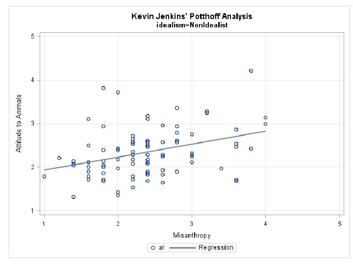
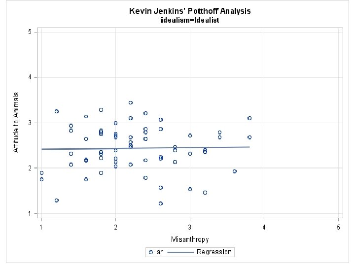
Get the Separate Regression Lines • Sort by groups. • Run the bivariate regressions Proc Sort; By Idealism; run; Proc Reg Simple Corr; Model ar=misanth; By Idealism; run; quit;

Get the Separate Regression Lines • For nonidealists, r =. 36, p <. 001, 95% CI [. 17, . 53] • For idealists, r =. 02, p =. 87, 95% CI [-. 23, . 27]

Prepare Plots Proc sgplot; scatter x = misanth y = ar; reg x = misanth y = ar; yaxis label='Attitude to Animals‘ grid values=(1 to 5 by 1); xaxis label='Misanthropy‘ grid values=(1 to 5 by 1); by idealism; run;

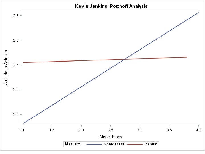
Another Plot proc sgplot; reg x = misanth y = ar / group = idealism nomarkers; yaxis label='Attitude to Animals'; xaxis label='Misanthropy'; run;

The Interaction Model, CGI Variable DF Parameter Estimate Intercept misanth idealism Mx. I 1 1 1. 62581 0. 30006 0. 77869 -0. 28472

Slope for Misanthropy • AR = 1. 626 + (. 300)Misanthropy + (. 779)Idealism_Group + (-. 285)Interaction. • If the moderator, Idealism_Group, has value zero, the slope is (. 300) Misanthropy +. 779(0) +(-. 285)(0)=. 300. • This (. 300) is a conditional slope. • It is the predicted increase in AR accompanying a one-point increase in misanthropy is. 3 given that idealism group (the moderator) has value zero (the nonidealists).

• the conditional effect of X on Y given a particular value of the moderator is the conditional slope for predictor X + the interaction slope times the value of the moderator. • Idealism Group as moderator, simple effect of misanthropy

Simple Slopes for Misanthropy • Idealism = 0 (nonidealists) • Each one point increase in Misanthropy leads to a. 3 point increase in AR. • Idealism = 1 (idealists) • Each one point increase in Misanthropy leads to a. 015 point increase in AR.

Change of Perspective • As with any two-way interaction, there are two different perspectives we can take. • We just looked at how the effects of Misanthropy differed between the two Idealism Groups. • Now we shall look at how the difference between the two Groups changes as the degree of Misanthropy increases.

Full Model Again • AR = 1. 626 + (. 300)Misanthropy + (. 779)Idealism + (-. 285)Interaction. • This is a conditional slope. • The predicted increase in AR accompanying a one-point increase in idealism (idealism groups were coded 0, 1) is. 779 given that misanthropy has value zero (which is an out of range value).

• Treating Misanthropy as the moderator, the simple slope for the effect of idealism group on AR is

Simple Slopes for Idealism • predict the difference between the two idealism groups (idealist minus nonidealist) when misanthropy = 1) • . 779 -. 285(1) =. 505. • If misanthropy = 4, the predicted difference in means is. 779 -. 285(4) = -. 361

Probing the Interaction • Same as simple effects analysis in ANOVA • Idealism group as the moderator • We have already shown (Slide 23) that the relationship between misanthropy and support for animal rights is greater (and significant) for nonidealists than for idealists (and not significant). • Idealism_Group moderates the effect of misanthropy.

Probing the Interaction • Change perspectives -- how does misanthropy moderate the relationship between idealism (group) and support of animal rights.

Analysis of Simple Slopes • Arbitrarily pick two or more values of misanthropy and compare the groups at those points. • The points are often 1 SD below the mean, and 1 SD above the mean. • Here, that would be misanthropy = 1. 65, 2. 32, and 2. 99.

Analysis of Simple Slopes • Arbitrarily pick two or more values of misanthropy and compare the groups at those points. • The points are often 1 SD below the mean, and 1 SD above the mean. • Here, that would be misanthropy = 1. 65, 2. 32, and 2. 99.

Testing the Simple Slopes • To test the null that mean AR does not differ between groups when misanthropy = 1. 65, we center the misanthropy scores around 1. 65, recompute the interaction term, and run the full model again. • We repeat this action with the scores centered around 2. 32 and then again centered around 2. 99.

The Code Data Centered; set kevin; Misanth. Low = misanth - 1. 65; Interact. Low = Misanth. Low * Idealism; Misanth. Mean = misanth - 2. 32; Interact. Mean = Misanth. Mean * Idealism; Misanth. High = misanth - 2. 99; Interact. High = Misanth. High * Idealism; Misanth 7 = misanth - 7; Interact 7 = Misanth 7 * Idealism;

proc reg; Low: model ar = Misanth. Low idealism Interact. Low; Mean: model ar = Misanth. Mean idealism Interact. Mean; High: model ar = Misanth. High idealism Interact. High; Way. Out: model ar = Misanth 7 idealism Interact 7; run; Quit;

Low Misanthropy When MIS is low, AR is significantly higher (by. 309) in the idealistic group than it is in the nonidealistic group.

Average Misanthropy • The groups do not differ significantly when MIS is average.

High Misanthropy • The groups do not differ significantly when MIS is High.

Way-Out Misanthropy • Misanthropy = 7 (an out-of-range value) • AR now significantly higher (by 1. 21) in the nonidealistic group. Parameter Estimates Variable DF Parameter Estimate Standard Error t Value Pr > |t| Intercept 1 3. 72620 0. 37657 9. 90 <. 0001 Misanth 7 1 0. 30006 0. 08059 3. 72 0. 0003 idealism 1 -1. 21436 0. 60066 -2. 02 0. 0450 Interact 7 1 -0. 28472 0. 12641 -2. 25 0. 0258

Process Hayes • Makes it way easier to do the moderation analysis • Does not do tests of coincidence and intercepts. • Bring the process. sas program into SAS and run it. • You have already read the data into the work file “kevin. ” • Hayes also provides a script to do the same in SPSS.

The SAS Macro %process (data=kevin, vars=ar misanth idealism, y=ar, x=idealism, m=misanth, model=1, jn=1, plot=1); • Data= points to the SAS data file • Vars= identifies the variables • Y= identifies the outcome variable • X= identifies the focal predictor variable • M= identifies the moderator variable • Model=1 identifies the simple moderation model – see the templates document

The SAS Macro %process (data=kevin, vars=ar misanth idealism, y=ar, x=idealism, m=misanth, model=1, jn=1, plot=1); • jn=1 invokes the Johnson-Neyman technique • Plot=1 requests the values for making a plot to visualize the interaction. • The code here is for Process version 2. The code is a little different for version 3.

The Templates Document • The link to it on Hayes’ site is now stale. • You can get it in the zip that you download with the Process software. • For the convenience of my students, a copy of the templates document is in Course Docs/Process Hayes.

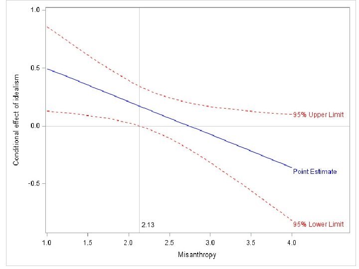
Johnson-Neyman Technique • Maps out the values of the moderator for which the effect of the focal predictor is significant versus those values for which it is not significant. • I’ll use idealism groups as the focal predictor and misanthropy as the moderator.

The Boundary • When misanthropy = 2. 1286 or less, the difference between the groups is statistically significant (higher for the idealists), otherwise it is not.

• If we were to extrapolate beyond misanthropy = 4, we would find a second region where the difference between the groups would be significant (with the mean higher for the nonidealists).

Johnson-Neyman Plot • Need to transfer some of the data from the “Conditional effect of X on Y at values of the moderator (M)” to a new data set. • Then use Proc Sgplot. • See the data and code in Potthoff_Process. sas

Process Version 3 %process (data=kevin, y=ar, x=idealism, w=misanth, model=1, jn=1, plot=1); • See the output here.

Don’t Confuse Tests of Slopes with Tests of Correlation Coefficients • If the slopes are the same across groups, the correlation coefficients (standardized slopes) may or may not. • If the correlation coefficients are the same across groups, the slopes may or may not be.

Different Slopes, Similar Correlations

Identical Slopes, Different Correlation Coefficients

Comparing the Groups on r • At SPSS and SAS programs for comparing Pearson correlations and OLS regression coefficients is the code for this analysis. • r is significant for nonidealists, not for idealists. • For more than two groups, use this chi square (also available at link above).

Idealism as the Moderator • %process (data=kevin, vars=ar misanth idealism, y=ar, x=misanth, m=idealism, model =1); • The test of the interaction is identical to that done when misanthropy was the moderator. Model coeff se t p LLCI ULCI constant 1. 6258 0. 1989 8. 1726 0. 0000 1. 2327 2. 0189 IDEALISM 0. 7787 0. 3024 2. 5753 0. 0110 0. 1812 1. 3761 MISANTH 0. 3001 0. 0806 3. 7230 0. 0003 0. 1408 0. 4593 -0. 2847 0. 1264 -2. 2523 0. 0258 -0. 5345 -0. 0349 INT_1

Tests of Intercepts & Slopes • The test of the main effect of Idealism is the test of intercepts. Earlier we got F = 6. 632, which is equivalent to t = 2. 575. • The test of the interaction is the test of slopes. Earlier we got F = 5. 073, which is equivalent to t = 2. 252.

• Among the nonidealists, the slope for predicting AR from misanthropy (. 3001) is significantly greater than zero. Among the idealists, the slope (. 0153) is not significantly different from zero. Conditional effect of X on Y at values of the moderator(s) IDEALISM Effect se t p LLCI ULCI 0. 0000 0. 3001 0. 0806 3. 7230 0. 0003 0. 1408 0. 4593 1. 0000 0. 0153 0. 0974 0. 1575 0. 8751 -0. 1771 0. 2078

Analysis of Covariance • You already know how to do this. • Just drop the interaction term from the model. • Here that would not be appropriate, as we have heterogeneity of regression.

A Couple of t Tests • You may also want to compare the groups on the Y (ignoring C) and/or C. • I have include those tests in the program. • This is redundant with the initial Proc Corr output (point biserial correlations).

SPSS • This analysis is easy to do with SPSS too. • See my handout. • You can do the analysis in a sequential fashion. • And get the partial F tests from SPSS, even with df > 1: Leave your calculator in the desk drawer.

Three Groups • Two dummy variables, G 1 and G 2 • Two interaction terms, G 1 C and G 2 C • To test the slopes you would see if the model fit were significantly reduced by simultaneously removing G 1 C and G 2 C. • That would be an F with two df in its numerator. • To test the intercepts, remove both G 1 and G 2

Let’s Go Fishing • Length = a + b Weight for flounder • Does the relationship differ across regions? – Pamlico Sound – Pamlico River – Tar River • Potthoff 3. sas and Potthoff 3. dat • Download and run.

Proc GLM • Proc GLM; class Location; o Model Length = Weight. SR|Location; • GLM creates the (2) dummy variables for you • And the (2) interaction terms.

Full Model Source DF Model 5 Error 745 Corrected 750 Total Sum of Mean F Value Squares Square 1927227. 450 385445. 490 3088. 09 92988. 508 124. 817 2020215. 957 Pr > F <. 0001

Covariate Only Model Proc GLM; class Location; model Length = Weight. SR / solution; Weights are significantly correlated with lengths, r 2 =. 95, F(1, 749) = 14, 544, p <. 001.

Test of Coincidence • On 4, 745 df, p <. 001 • The lines are not coincident.

Look at Full Model • The slopes do not differ significantly, F(2, 745) = 1. 63, p =. 20. • The intercepts do differ significantly, F(2, 745) = 4. 90, p =. 008. • Since the slopes do not differ significantly • But the intercepts do, • The group means must differ. • Drop the interaction from the model (ANCOV)

Source DF Type III SS Mean Square F Value Pr > F Weight. SR 1 692152. 6411 5545. 35 <. 0001 Location 2 Weight. SR* 2 Location 1223. 2971 407. 5286 4. 90 1. 63 611. 6486 203. 7643 0. 0077 0. 1961

Analysis of Covariance • Location significantly affects mean length of flounder, after adjusting for the effect of weight (LSMEANS).

Unadjusted Means (notice the different pattern)