COMP 171 Fall 2005 Graph Graph Slide 2

COMP 171 Fall 2005 Graph

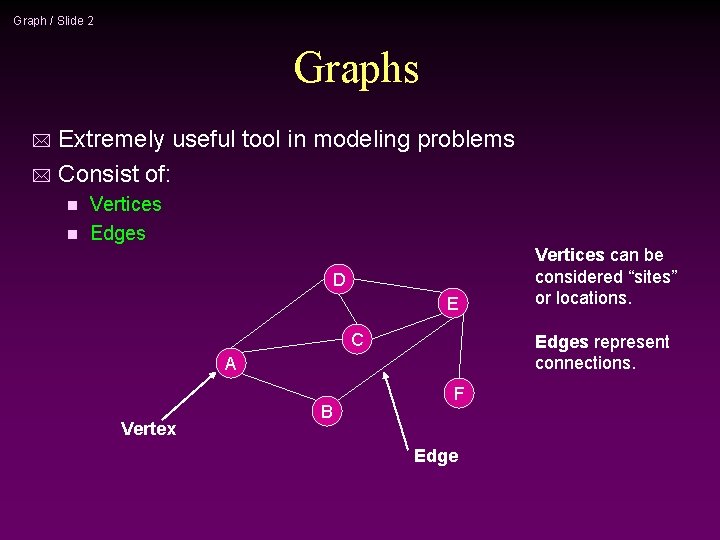
Graph / Slide 2 Graphs Extremely useful tool in modeling problems * Consist of: * Vertices n Edges n D E C Edges represent connections. A Vertex B Vertices can be considered “sites” or locations. F Edge

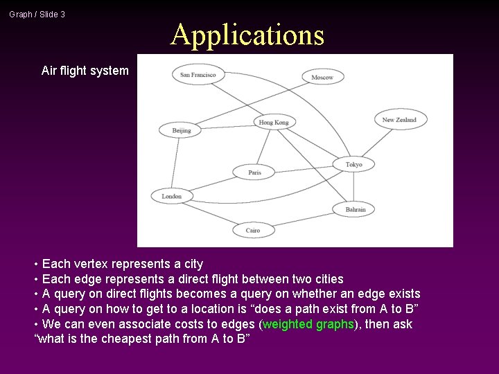
Graph / Slide 3 Applications Air flight system • Each vertex represents a city • Each edge represents a direct flight between two cities • A query on direct flights becomes a query on whether an edge exists • A query on how to get to a location is “does a path exist from A to B” • We can even associate costs to edges (weighted graphs), then ask “what is the cheapest path from A to B”

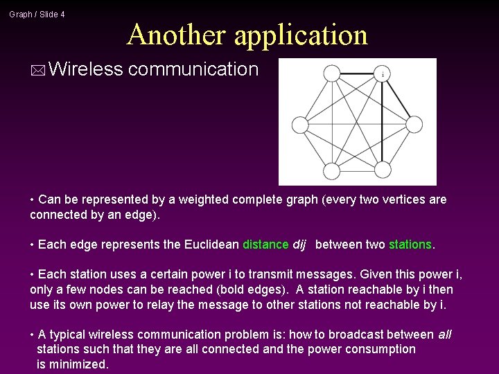
Graph / Slide 4 * Wireless Another application communication • Can be represented by a weighted complete graph (every two vertices are connected by an edge). • Each edge represents the Euclidean distance dij between two stations. • Each station uses a certain power i to transmit messages. Given this power i, only a few nodes can be reached (bold edges). A station reachable by i then use its own power to relay the message to other stations not reachable by i. • A typical wireless communication problem is: how to broadcast between all stations such that they are all connected and the power consumption is minimized.

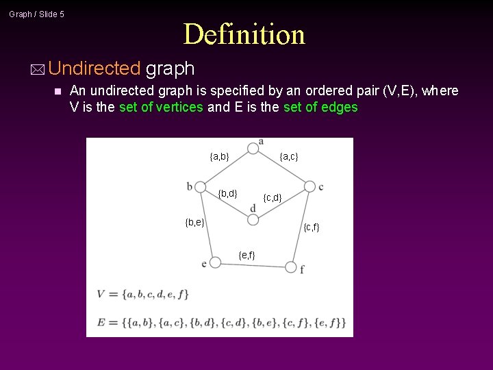
Graph / Slide 5 Definition * Undirected n graph An undirected graph is specified by an ordered pair (V, E), where V is the set of vertices and E is the set of edges {a, b} {a, c} {b, d} {c, d} {b, e} {c, f} {e, f}

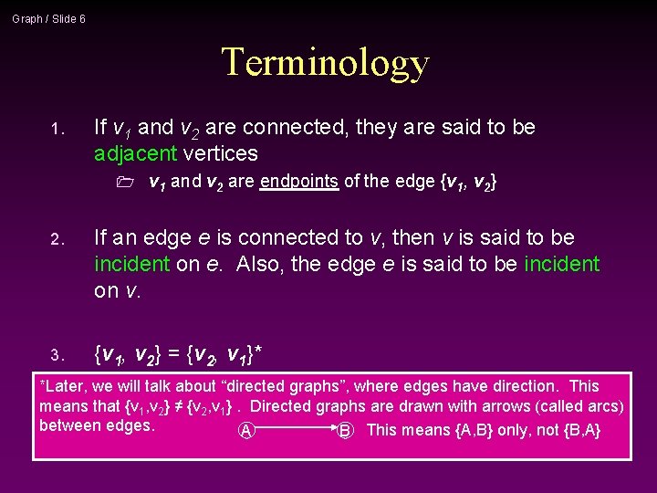
Graph / Slide 6 Terminology 1. If v 1 and v 2 are connected, they are said to be adjacent vertices 1 v 1 and v 2 are endpoints of the edge {v 1, v 2} 2. If an edge e is connected to v, then v is said to be incident on e. Also, the edge e is said to be incident on v. 3. {v 1, v 2} = {v 2, v 1}* *Later, we will talk about “directed graphs”, where edges have direction. This means that {v 1, v 2} ≠ {v 2, v 1}. Directed graphs are drawn with arrows (called arcs) between edges. A B This means {A, B} only, not {B, A}

Graph / Slide 7 Graph Representation * Two popular computer representations of a graph. Both represent the vertex set and the edge set, but in different ways. 1. Adjacency Matrix Use a 2 D matrix to represent the graph 2. Adjacency List Use a 1 D array of linked lists

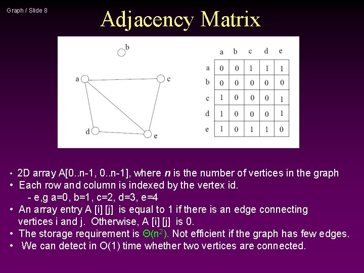
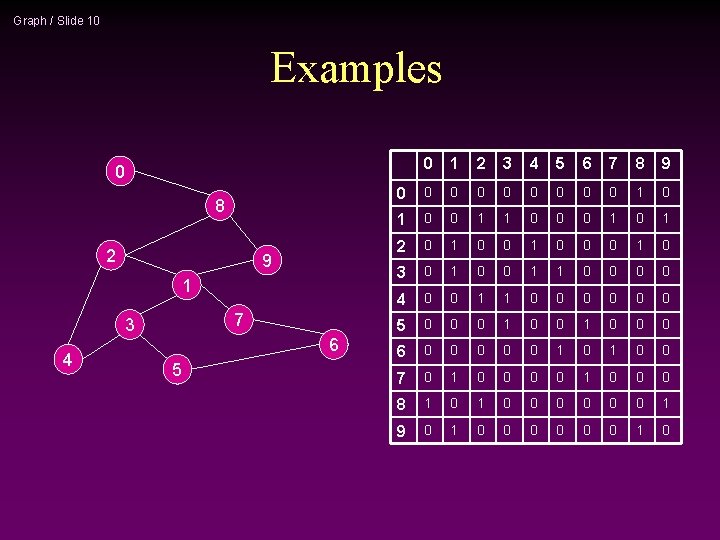
Graph / Slide 8 • • • Adjacency Matrix 2 D array A[0. . n-1, 0. . n-1], where n is the number of vertices in the graph Each row and column is indexed by the vertex id. - e, g a=0, b=1, c=2, d=3, e=4 An array entry A [i] [j] is equal to 1 if there is an edge connecting vertices i and j. Otherwise, A [i] [j] is 0. The storage requirement is Θ(n 2). Not efficient if the graph has few edges. We can detect in O(1) time whether two vertices are connected.

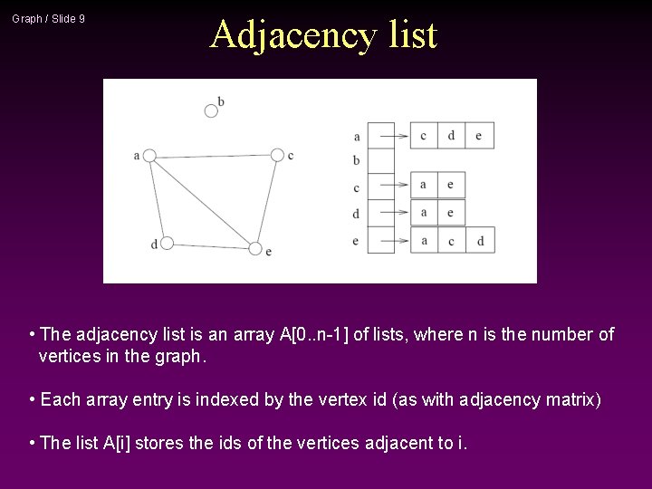
Graph / Slide 9 Adjacency list • The adjacency list is an array A[0. . n-1] of lists, where n is the number of vertices in the graph. • Each array entry is indexed by the vertex id (as with adjacency matrix) • The list A[i] stores the ids of the vertices adjacent to i.

Graph / Slide 10 Examples 0 1 2 3 4 5 6 7 8 9 0 0 0 0 0 1 1 0 0 0 1 2 0 1 0 0 0 1 0 3 0 1 0 0 1 1 0 0 4 0 0 1 1 0 0 0 5 0 0 0 1 0 0 0 6 0 0 0 1 0 0 7 0 1 0 0 0 8 1 0 0 0 0 1 9 0 1 0 0 8 2 9 1 7 3 4 6 5

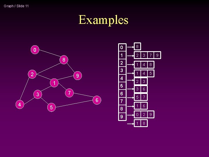
Graph / Slide 11 Examples 0 8 2 2 3 7 2 1 4 8 1 4 5 2 3 3 6 5 7 1 6 0 2 1 8 5 7 6 6 5 1 4 8 3 9 3 0 7 8 9 9 9

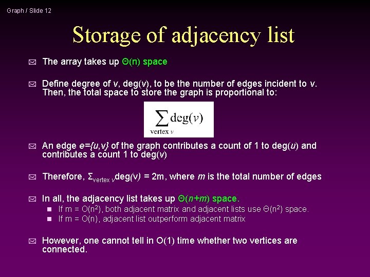
Graph / Slide 12 Storage of adjacency list * The array takes up Θ(n) space * Define degree of v, deg(v), to be the number of edges incident to v. Then, the total space to store the graph is proportional to: * An edge e={u, v} of the graph contributes a count of 1 to deg(u) and contributes a count 1 to deg(v) * Therefore, Σvertex vdeg(v) = 2 m, where m is the total number of edges * In all, the adjacency list takes up Θ(n+m) space. n n * If m = O(n 2), both adjacent matrix and adjacent lists use Θ(n 2) space. If m = O(n), adjacent list outperform adjacent matrix However, one cannot tell in O(1) time whether two vertices are connected.

Graph / Slide 13 Adjacency Lists vs. Matrix * Adjacency Lists n n * More compact than adjacency matrices if graph has few edges Requires more time to find if an edge exists Adjacency Matrix Always require n 2 space 1 This can waste a lot of space if the number of edges are sparse n Can quickly find if an edge exists n

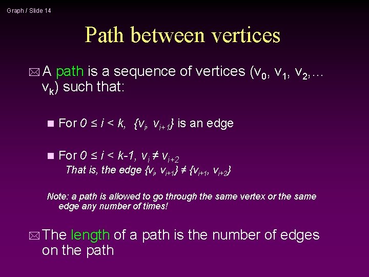
Graph / Slide 14 Path between vertices *A path is a sequence of vertices (v 0, v 1, v 2, … vk) such that: n For 0 ≤ i < k, {vi, vi+1} is an edge n For 0 ≤ i < k-1, vi ≠ vi+2 That is, the edge {vi, vi+1} ≠ {vi+1, vi+2} Note: a path is allowed to go through the same vertex or the same edge any number of times! * The length of a path is the number of edges on the path

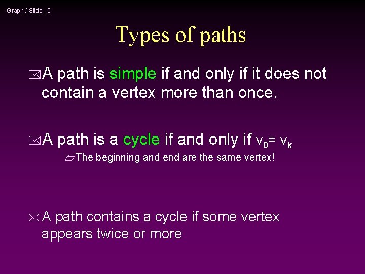
Graph / Slide 15 Types of paths *A path is simple if and only if it does not contain a vertex more than once. *A path is a cycle if and only if v 0= vk 1 The *A beginning and end are the same vertex! path contains a cycle if some vertex appears twice or more

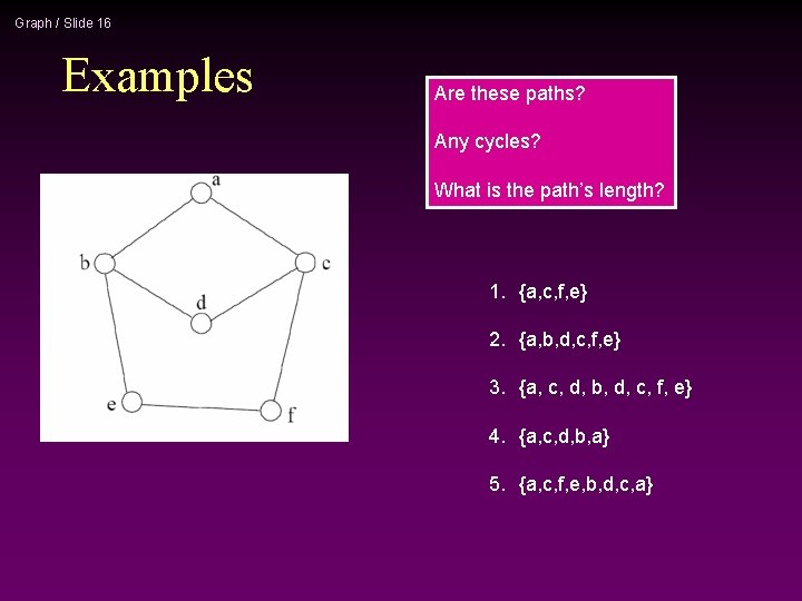
Graph / Slide 16 Examples Are these paths? Any cycles? What is the path’s length? 1. {a, c, f, e} 2. {a, b, d, c, f, e} 3. {a, c, d, b, d, c, f, e} 4. {a, c, d, b, a} 5. {a, c, f, e, b, d, c, a}

Graph / Slide 17 * Graph Traversal Application example Given a graph representation and a vertex s in the graph n Find all paths from s to other vertices n * Two * common graph traversal algorithms 1 Breadth-First Search (BFS) l Find the shortest paths in an unweighted graph 1 Depth-First Search (DFS) l Topological sort l Find strongly connected components Let’s first look at BFS. . .

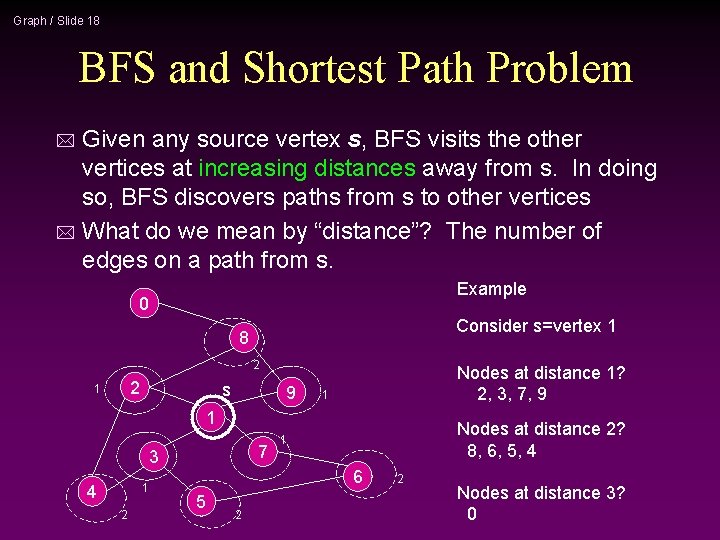
Graph / Slide 18 BFS and Shortest Path Problem Given any source vertex s, BFS visits the other vertices at increasing distances away from s. In doing so, BFS discovers paths from s to other vertices * What do we mean by “distance”? The number of edges on a path from s. * Example 0 Consider s=vertex 1 8 2 2 1 s 9 Nodes at distance 1? 2, 3, 7, 9 1 1 7 3 1 4 2 Nodes at distance 2? 8, 6, 5, 4 1 6 5 2 2 Nodes at distance 3? 0

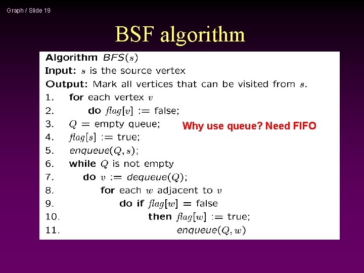
Graph / Slide 19 BSF algorithm Why use queue? Need FIFO

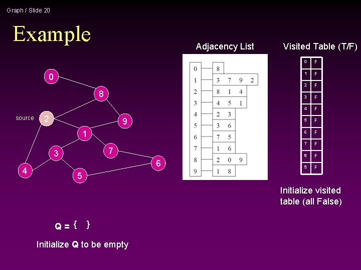
Graph / Slide 20 Example Adjacency List 0 8 source 2 9 1 7 3 4 6 Visited Table (T/F) 0 F 1 F 2 F 3 F 4 F 5 F 6 F 7 F 8 F 9 F 5 Initialize visited table (all False) Q= { } Initialize Q to be empty

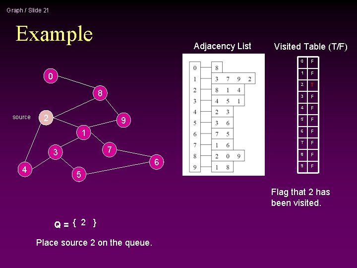
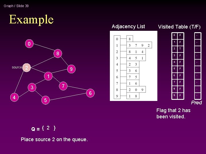
Graph / Slide 21 Example Adjacency List 0 8 source 2 9 1 7 3 4 6 Visited Table (T/F) 0 F 1 F 2 T 3 F 4 F 5 F 6 F 7 F 8 F 9 F 5 Flag that 2 has been visited. Q= { 2 } Place source 2 on the queue.

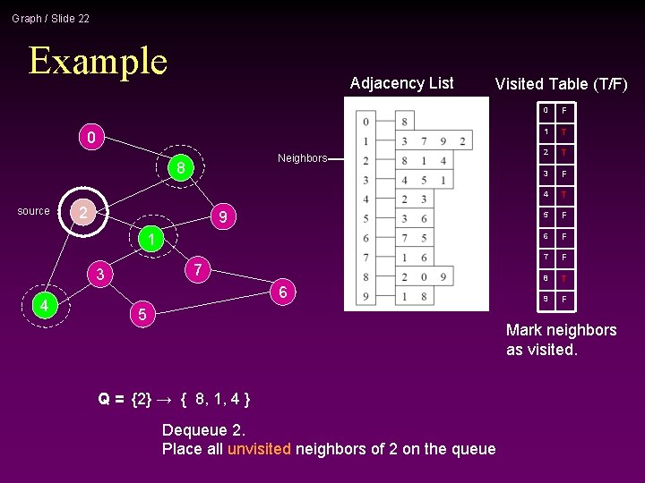
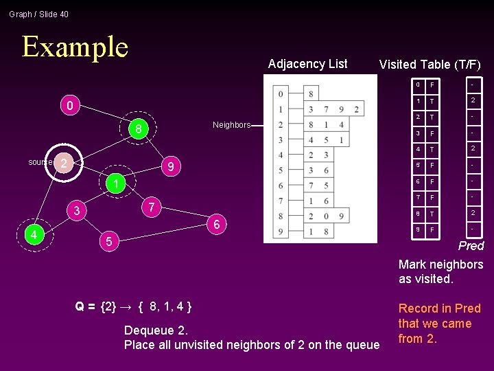
Graph / Slide 22 Example Adjacency List Visited Table (T/F) 0 Neighbors 8 source 2 9 1 7 3 4 6 5 0 F 1 T 2 T 3 F 4 T 5 F 6 F 7 F 8 T 9 F Mark neighbors as visited. Q = {2} → { 8, 1, 4 } Dequeue 2. Place all unvisited neighbors of 2 on the queue

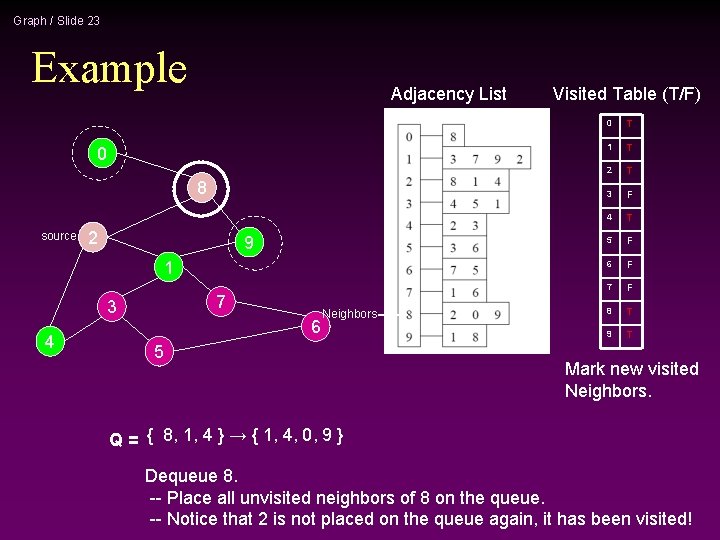
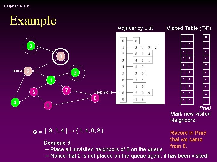
Graph / Slide 23 Example Adjacency List 0 8 source 2 9 1 7 3 4 6 Neighbors 5 Visited Table (T/F) 0 T 1 T 2 T 3 F 4 T 5 F 6 F 7 F 8 T 9 T Mark new visited Neighbors. Q = { 8, 1, 4 } → { 1, 4, 0, 9 } Dequeue 8. -- Place all unvisited neighbors of 8 on the queue. -- Notice that 2 is not placed on the queue again, it has been visited!

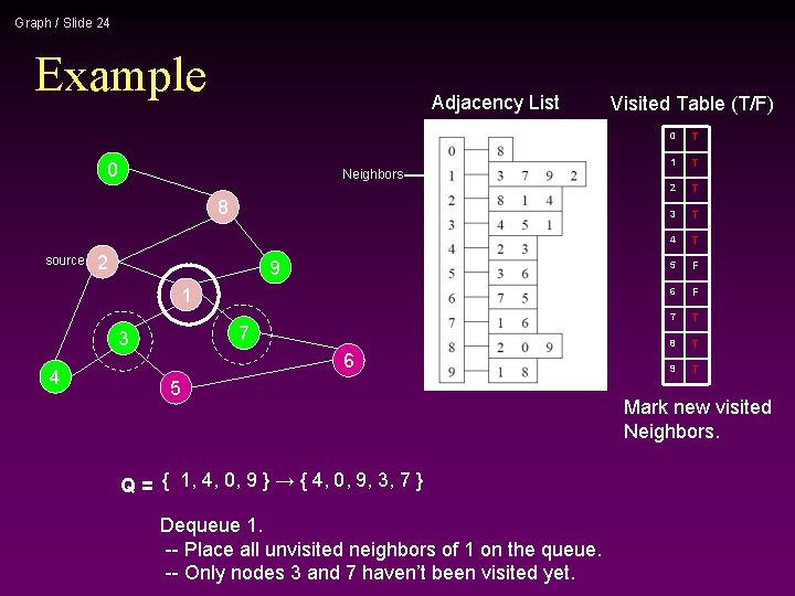
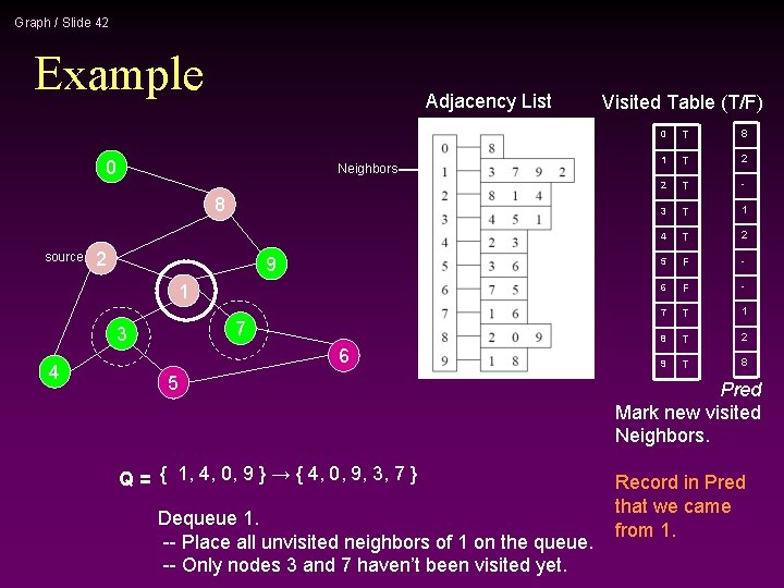
Graph / Slide 24 Example Adjacency List 0 Neighbors 8 source 2 9 1 7 3 4 6 5 Q = { 1, 4, 0, 9 } → { 4, 0, 9, 3, 7 } Dequeue 1. -- Place all unvisited neighbors of 1 on the queue. -- Only nodes 3 and 7 haven’t been visited yet. Visited Table (T/F) 0 T 1 T 2 T 3 T 4 T 5 F 6 F 7 T 8 T 9 T Mark new visited Neighbors.

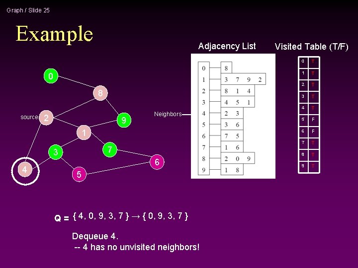
Graph / Slide 25 Example Adjacency List 0 8 source 2 9 Neighbors 1 7 3 4 6 5 Q = { 4, 0, 9, 3, 7 } → { 0, 9, 3, 7 } Dequeue 4. -- 4 has no unvisited neighbors! Visited Table (T/F) 0 T 1 T 2 T 3 T 4 T 5 F 6 F 7 T 8 T 9 T

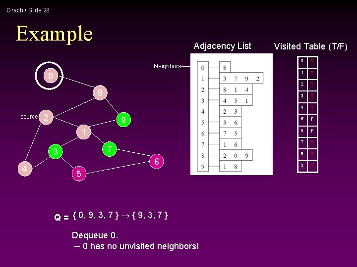
Graph / Slide 26 Example Adjacency List Neighbors 0 8 source 2 9 1 7 3 4 6 5 Q = { 0, 9, 3, 7 } → { 9, 3, 7 } Dequeue 0. -- 0 has no unvisited neighbors! Visited Table (T/F) 0 T 1 T 2 T 3 T 4 T 5 F 6 F 7 T 8 T 9 T

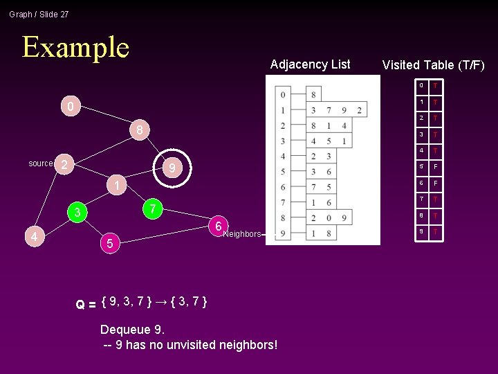
Graph / Slide 27 Example Adjacency List 0 8 source 2 9 1 7 3 4 5 6 Neighbors Q = { 9, 3, 7 } → { 3, 7 } Dequeue 9. -- 9 has no unvisited neighbors! Visited Table (T/F) 0 T 1 T 2 T 3 T 4 T 5 F 6 F 7 T 8 T 9 T

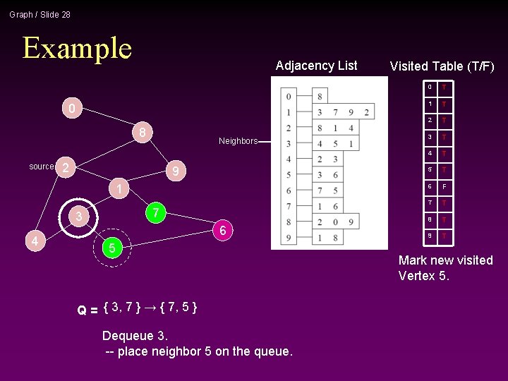
Graph / Slide 28 Example Adjacency List 0 8 source Neighbors 2 9 1 7 3 4 6 5 Q = { 3, 7 } → { 7, 5 } Dequeue 3. -- place neighbor 5 on the queue. Visited Table (T/F) 0 T 1 T 2 T 3 T 4 T 5 T 6 F 7 T 8 T 9 T Mark new visited Vertex 5.

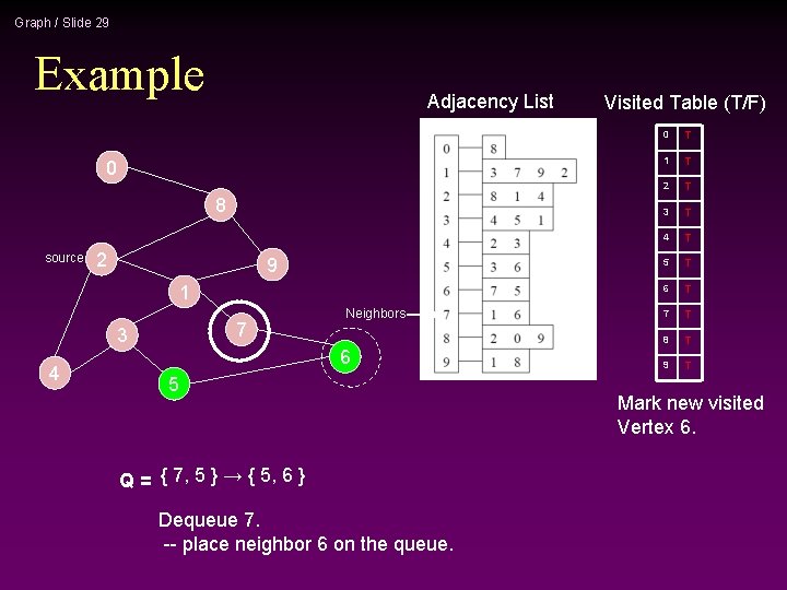
Graph / Slide 29 Example Adjacency List 0 8 source 2 9 1 7 3 4 Neighbors 6 5 Q = { 7, 5 } → { 5, 6 } Dequeue 7. -- place neighbor 6 on the queue. Visited Table (T/F) 0 T 1 T 2 T 3 T 4 T 5 T 6 T 7 T 8 T 9 T Mark new visited Vertex 6.

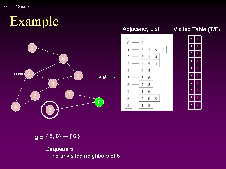
Graph / Slide 30 Example Adjacency List 0 8 source 2 9 Neighbors 1 7 3 4 6 5 Q = { 5, 6} → { 6 } Dequeue 5. -- no unvisited neighbors of 5. Visited Table (T/F) 0 T 1 T 2 T 3 T 4 T 5 T 6 T 7 T 8 T 9 T

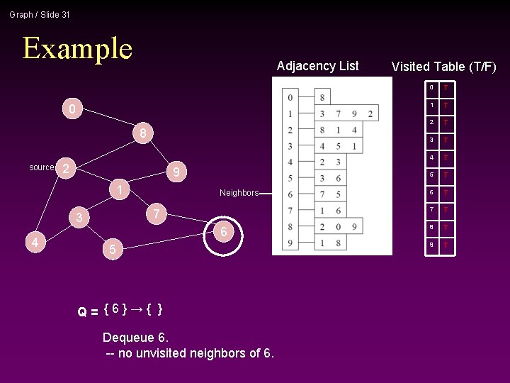
Graph / Slide 31 Example Adjacency List 0 8 source 2 9 1 7 3 4 Neighbors 6 5 Q= {6}→{ } Dequeue 6. -- no unvisited neighbors of 6. Visited Table (T/F) 0 T 1 T 2 T 3 T 4 T 5 T 6 T 7 T 8 T 9 T

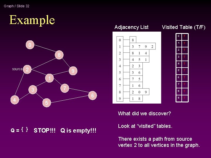
Graph / Slide 32 Example Adjacency List Visited Table (T/F) 0 8 source 2 9 1 7 3 4 6 0 T 1 T 2 T 3 T 4 T 5 T 6 T 7 T 8 T 9 T 5 What did we discover? Q= { } STOP!!! Q is empty!!! Look at “visited” tables. There exists a path from source vertex 2 to all vertices in the graph.

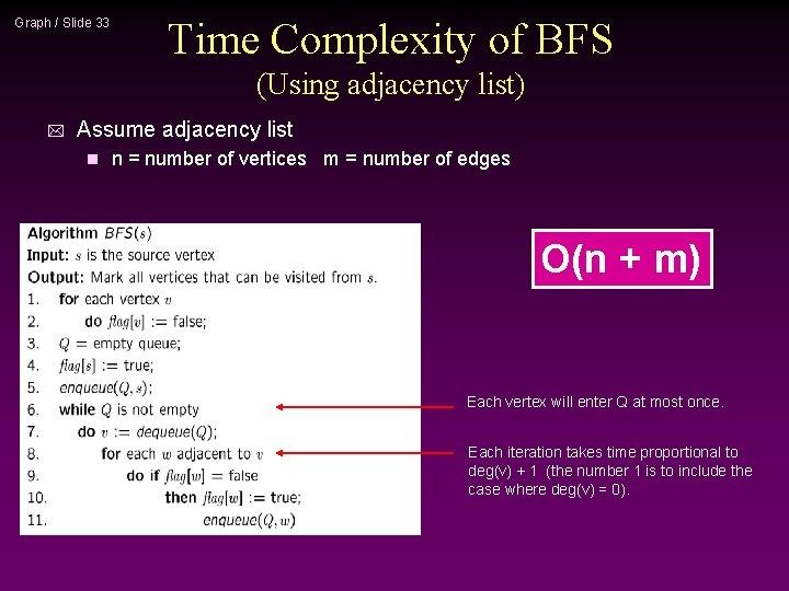
Graph / Slide 33 Time Complexity of BFS (Using adjacency list) * Assume adjacency list n n = number of vertices m = number of edges O(n + m) Each vertex will enter Q at most once. Each iteration takes time proportional to deg(v) + 1 (the number 1 is to include the case where deg(v) = 0).

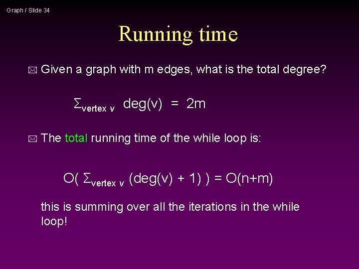
Graph / Slide 34 Running time * Given a graph with m edges, what is the total degree? Σvertex v deg(v) = 2 m * The total running time of the while loop is: O( Σvertex v (deg(v) + 1) ) = O(n+m) this is summing over all the iterations in the while loop!

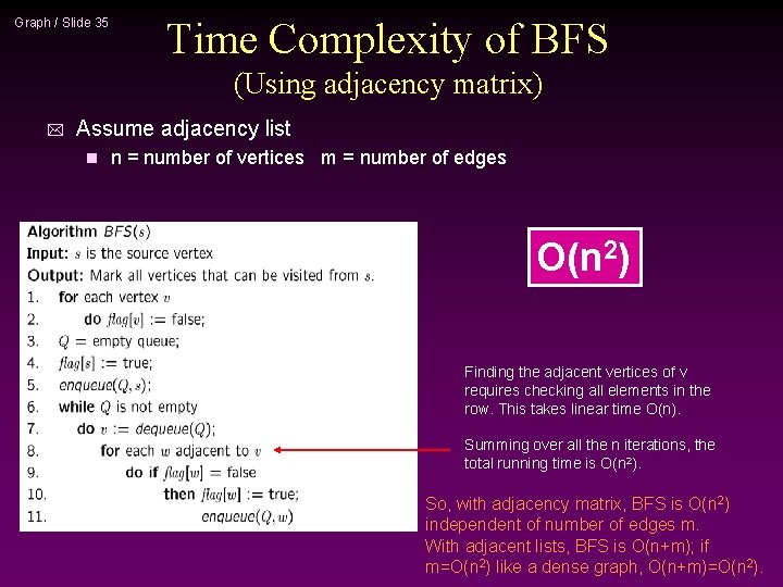
Graph / Slide 35 Time Complexity of BFS (Using adjacency matrix) * Assume adjacency list n n = number of vertices m = number of edges O(n 2) Finding the adjacent vertices of v requires checking all elements in the row. This takes linear time O(n). Summing over all the n iterations, the total running time is O(n 2). So, with adjacency matrix, BFS is O(n 2) independent of number of edges m. With adjacent lists, BFS is O(n+m); if m=O(n 2) like a dense graph, O(n+m)=O(n 2).

Graph / Slide 36 Shortest Path Recording * BFS we saw only tells us whether a path exists from source s, to other vertices v. It doesn’t tell us the path! n We need to modify the algorithm to record the path. n * How can we do that? Note: we do not know which vertices lie on this path until we reach v! n Efficient solution: n 1 Use an additional array pred[0. . n-1] 1 Pred[w] = v means that vertex w was visited from v

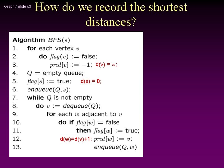
Graph / Slide 37 BFS + Path Finding initialize all pred[v] to -1 Record where you came from

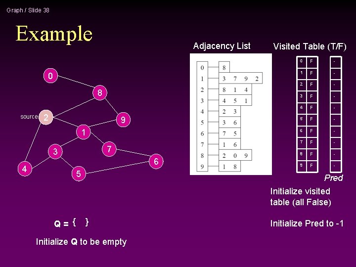
Graph / Slide 38 Example Adjacency List 0 8 source 2 9 1 7 3 4 6 5 Visited Table (T/F) 0 F - 1 F - 2 F - 3 F - 4 F - 5 F - 6 F - 7 F - 8 F - 9 F - Pred Initialize visited table (all False) Q= { } Initialize Q to be empty Initialize Pred to -1

Graph / Slide 39 Example Adjacency List 0 8 source 2 9 1 7 3 4 6 Visited Table (T/F) 0 F - 1 F - 2 T - 3 F - 4 F - 5 F - 6 F - 7 F - 8 F - 9 F - 5 Pred Flag that 2 has been visited. Q= { 2 } Place source 2 on the queue.

Graph / Slide 40 Example Adjacency List Visited Table (T/F) 0 Neighbors 8 source 2 9 1 7 3 4 6 5 0 F - 1 T 2 2 T - 3 F - 4 T 2 5 F - 6 F - 7 F - 8 T 2 9 F - Pred Mark neighbors as visited. Q = {2} → { 8, 1, 4 } Dequeue 2. Place all unvisited neighbors of 2 on the queue Record in Pred that we came from 2.

Graph / Slide 41 Example Adjacency List 0 8 source 2 9 1 7 3 4 Neighbors 6 5 Q = { 8, 1, 4 } → { 1, 4, 0, 9 } Visited Table (T/F) 0 T 8 1 T 2 2 T - 3 F - 4 T 2 5 F - 6 F - 7 F - 8 T 2 9 T 8 Pred Mark new visited Neighbors. Record in Pred that we came from 8. Dequeue 8. -- Place all unvisited neighbors of 8 on the queue. -- Notice that 2 is not placed on the queue again, it has been visited!

Graph / Slide 42 Example Adjacency List 0 Neighbors 8 source 2 9 1 7 3 4 6 5 Q = { 1, 4, 0, 9 } → { 4, 0, 9, 3, 7 } Dequeue 1. -- Place all unvisited neighbors of 1 on the queue. -- Only nodes 3 and 7 haven’t been visited yet. Visited Table (T/F) 0 T 8 1 T 2 2 T - 3 T 1 4 T 2 5 F - 6 F - 7 T 1 8 T 2 9 T 8 Pred Mark new visited Neighbors. Record in Pred that we came from 1.

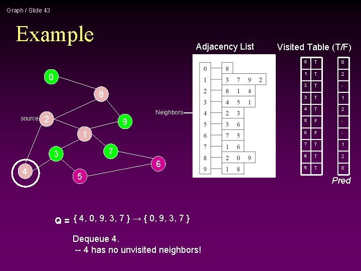
Graph / Slide 43 Example Adjacency List 0 8 source Neighbors 2 9 1 7 3 4 6 5 Q = { 4, 0, 9, 3, 7 } → { 0, 9, 3, 7 } Dequeue 4. -- 4 has no unvisited neighbors! Visited Table (T/F) 0 T 8 1 T 2 2 T - 3 T 1 4 T 2 5 F - 6 F - 7 T 1 8 T 2 9 T 8 Pred

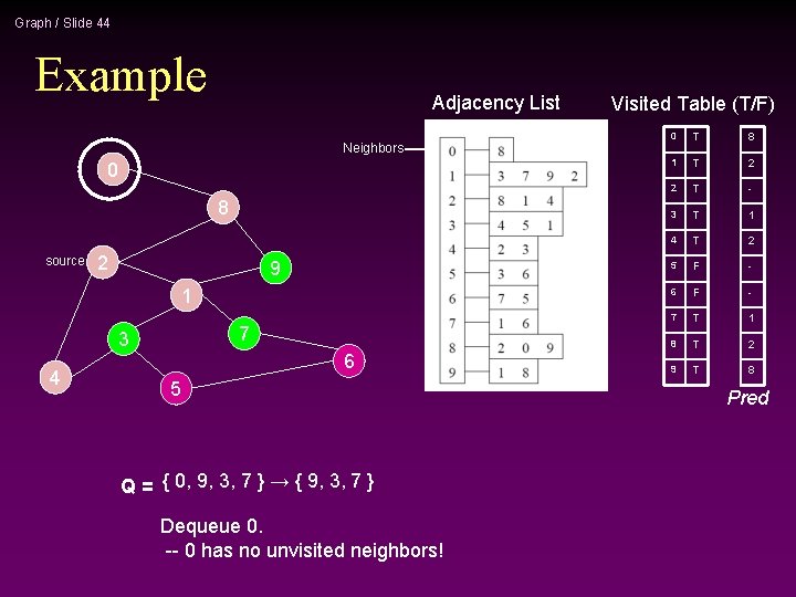
Graph / Slide 44 Example Adjacency List Neighbors 0 8 source 2 9 1 7 3 4 6 5 Q = { 0, 9, 3, 7 } → { 9, 3, 7 } Dequeue 0. -- 0 has no unvisited neighbors! Visited Table (T/F) 0 T 8 1 T 2 2 T - 3 T 1 4 T 2 5 F - 6 F - 7 T 1 8 T 2 9 T 8 Pred

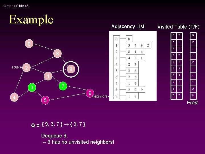
Graph / Slide 45 Example Adjacency List 0 8 source 2 9 1 7 3 4 5 6 Neighbors Q = { 9, 3, 7 } → { 3, 7 } Dequeue 9. -- 9 has no unvisited neighbors! Visited Table (T/F) 0 T 8 1 T 2 2 T - 3 T 1 4 T 2 5 F - 6 F - 7 T 1 8 T 2 9 T 8 Pred

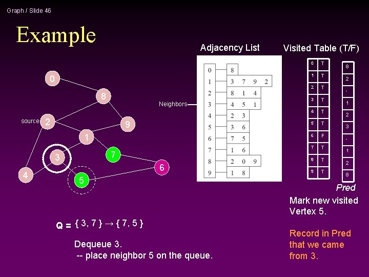
Graph / Slide 46 Example Adjacency List 0 8 source Neighbors 2 9 1 7 3 4 6 5 Q = { 3, 7 } → { 7, 5 } Dequeue 3. -- place neighbor 5 on the queue. Visited Table (T/F) 0 T 1 T 2 T 3 T 4 T 5 T 6 F 7 T 8 T 9 T 8 2 1 2 3 1 2 8 Pred Mark new visited Vertex 5. Record in Pred that we came from 3.

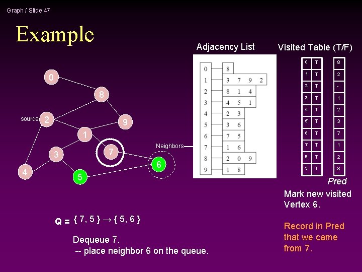
Graph / Slide 47 Example Adjacency List 0 8 source 2 9 1 7 3 4 Neighbors 6 5 Q = { 7, 5 } → { 5, 6 } Dequeue 7. -- place neighbor 6 on the queue. Visited Table (T/F) 0 T 8 1 T 2 2 T - 3 T 1 4 T 2 5 T 3 6 T 7 7 T 1 8 T 2 9 T 8 Pred Mark new visited Vertex 6. Record in Pred that we came from 7.

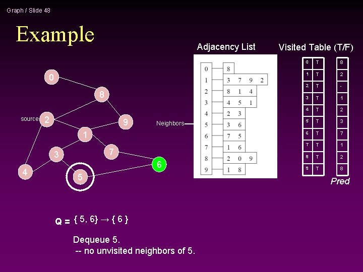
Graph / Slide 48 Example Adjacency List 0 8 source 2 9 Neighbors 1 7 3 4 6 5 Q = { 5, 6} → { 6 } Dequeue 5. -- no unvisited neighbors of 5. Visited Table (T/F) 0 T 8 1 T 2 2 T - 3 T 1 4 T 2 5 T 3 6 T 7 7 T 1 8 T 2 9 T 8 Pred

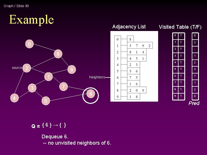
Graph / Slide 49 Example Adjacency List 0 8 source 2 9 1 7 3 4 Neighbors 6 5 Q= {6}→{ } Dequeue 6. -- no unvisited neighbors of 6. Visited Table (T/F) 0 T 8 1 T 2 2 T - 3 T 1 4 T 2 5 T 3 6 T 7 7 T 1 8 T 2 9 T 8 Pred

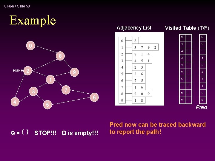
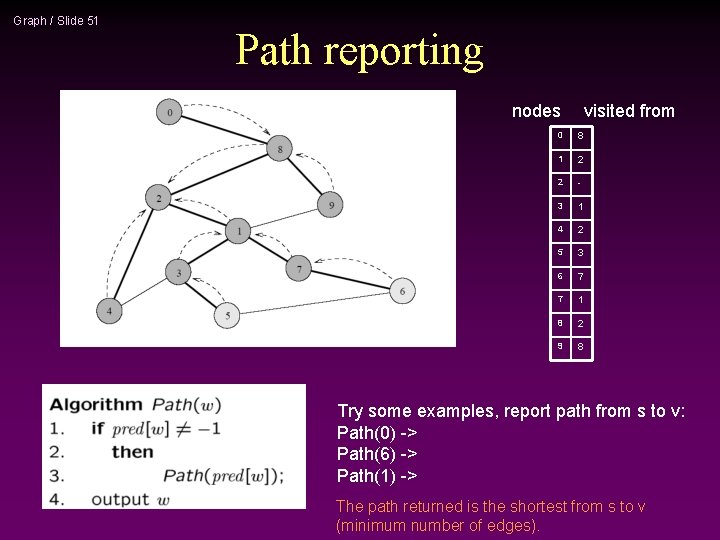
Graph / Slide 50 Example Adjacency List 0 8 source 2 9 1 7 3 4 Q= { } 6 5 STOP!!! Q is empty!!! Visited Table (T/F) 0 T 8 1 T 2 2 T - 3 T 1 4 T 2 5 T 3 6 T 7 7 T 1 8 T 2 9 T 8 Pred now can be traced backward to report the path!

Graph / Slide 51 Path reporting nodes visited from 0 8 1 2 2 - 3 1 4 2 5 3 6 7 7 1 8 2 9 8 Try some examples, report path from s to v: Path(0) -> Path(6) -> Path(1) -> The path returned is the shortest from s to v (minimum number of edges).

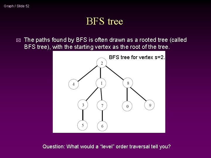
Graph / Slide 52 BFS tree * The paths found by BFS is often drawn as a rooted tree (called BFS tree), with the starting vertex as the root of the tree. BFS tree for vertex s=2. Question: What would a “level” order traversal tell you?

Graph / Slide 53 How do we record the shortest distances? d(v) = ; d(s) = 0; d(w)=d(v)+1;

Graph / Slide 54 Application of BFS * * One application concerns how to find connected components in a graph If a graph has more than one connected components, BFS builds a BFS-forest (not just BFS-tree)! n Each tree in the forest is a connected component.