Communication Entropy In thermodynamics entropy is a measure


- Slides: 49

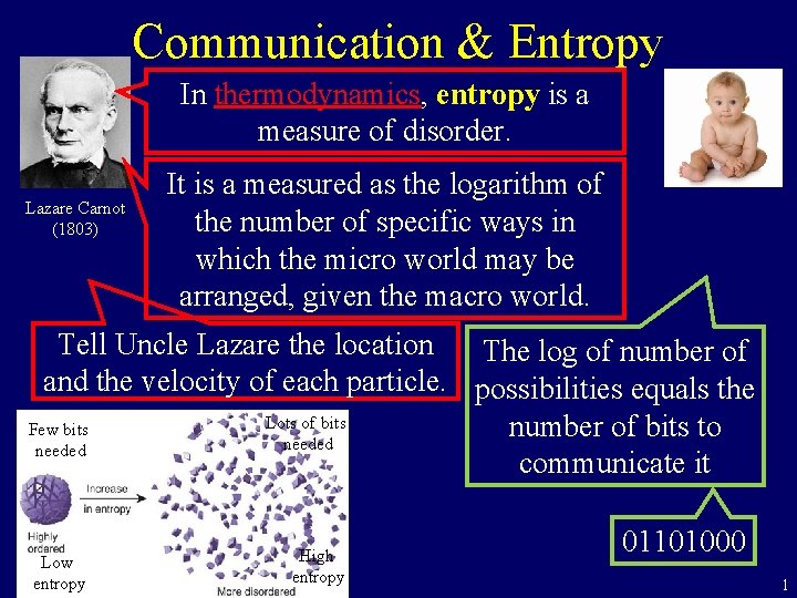
Communication & Entropy In thermodynamics, entropy is a measure of disorder. Lazare Carnot (1803) It is a measured as the logarithm of the number of specific ways in which the micro world may be arranged, given the macro world. Tell Uncle Lazare the location The log of number of and the velocity of each particle. possibilities equals the Lots of bits Few bits number of bits to needed communicate it Low entropy High entropy 01101000 1

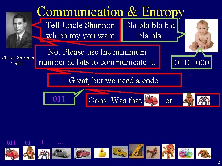
Communication & Entropy Tell Uncle Shannon which toy you want Claude Shannon (1948) Bla bla bla bla No. Please use the minimum number of bits to communicate it. 01101000 Great, but we need a code. 011 01 1 Oops. Was that or … 2

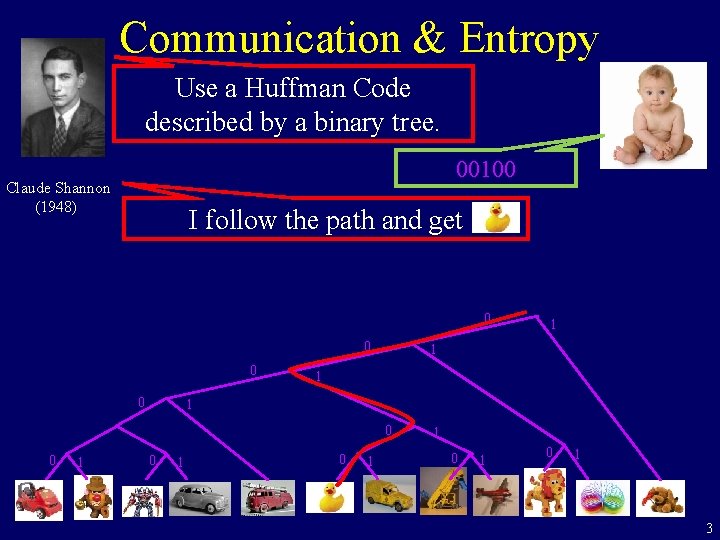
Communication & Entropy Use a Huffman Code described by a binary tree. 00100 Claude Shannon (1948) I follow the path and get 0 0 1 1 1 0 0 1 1 0 1 0 1 3

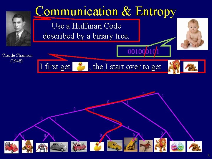
Communication & Entropy Use a Huffman Code described by a binary tree. Claude Shannon (1948) 00101 I first get , the I start over to get 0 0 1 1 1 0 0 1 1 0 1 0 1 4

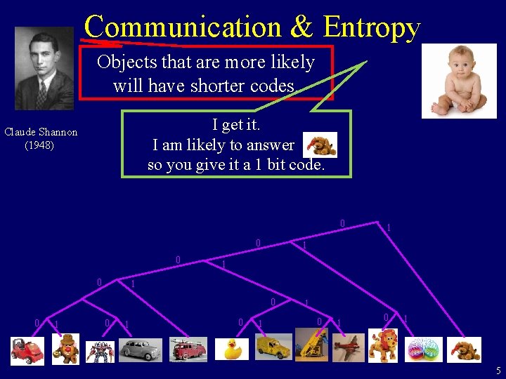
Communication & Entropy Objects that are more likely will have shorter codes. I get it. I am likely to answer. so you give it a 1 bit code. Claude Shannon (1948) 0 0 1 1 1 0 0 1 1 0 1 0 1 5

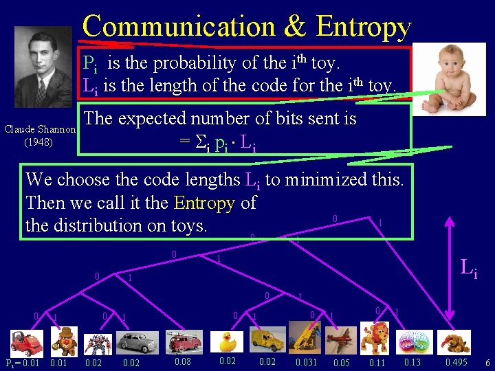
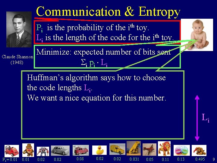
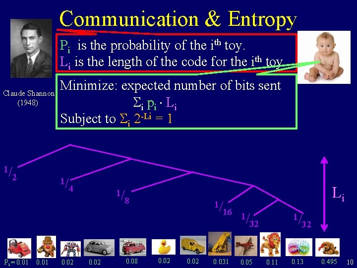
Communication & Entropy Pi is the probability of the ith toy. Li is the length of the code for the ith toy. Claude Shannon (1948) The expected number of bits sent is = i pi Li We choose the code lengths Li to minimized this. Then we call it the Entropy of 0 1 the distribution on toys. 0 1 0 0 1 Li 1 0 0 Pi = 0. 01 0 1 0. 02 0. 08 0. 02 1 0. 02 0. 031 1 0. 05 0 0. 11 1 0. 13 0. 495 6

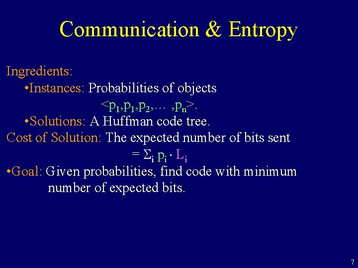
Communication & Entropy Ingredients: • Instances: Probabilities of objects <p 1, p 2, … , pn>. • Solutions: A Huffman code tree. Cost of Solution: The expected number of bits sent = i pi Li • Goal: Given probabilities, find code with minimum number of expected bits. 7

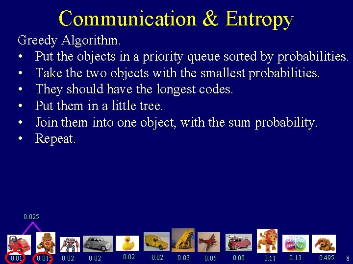
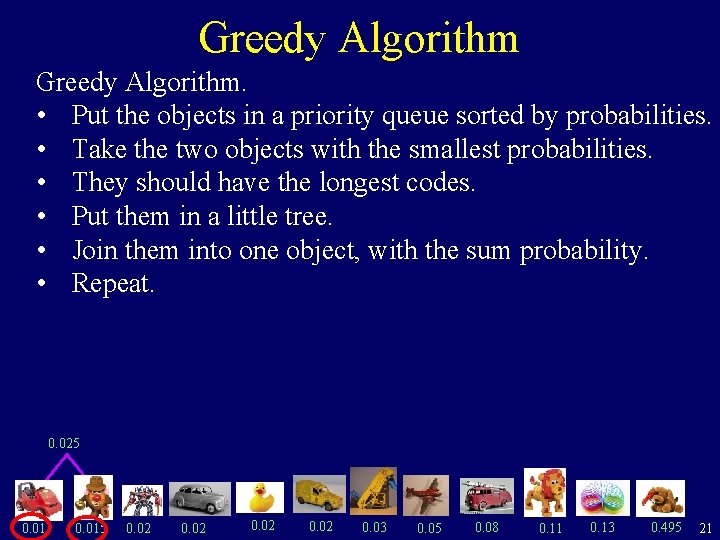
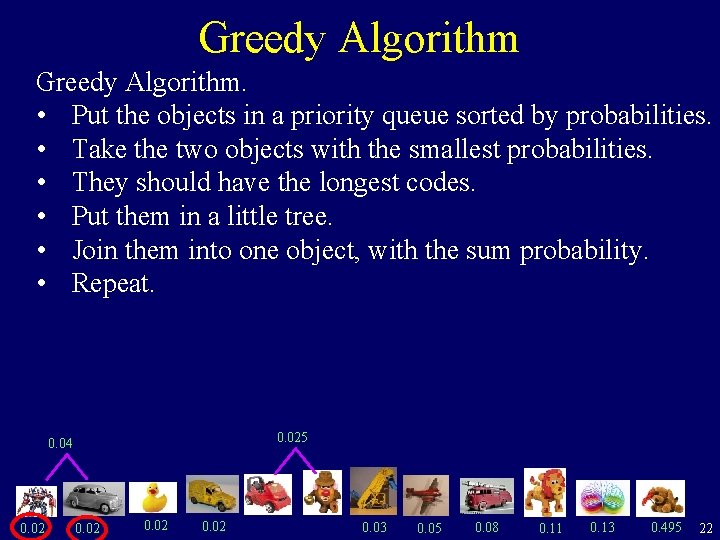
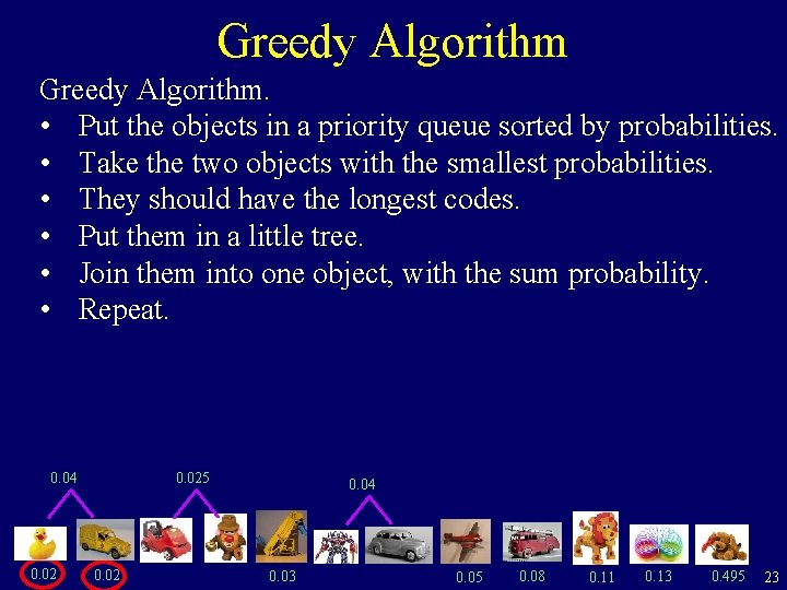
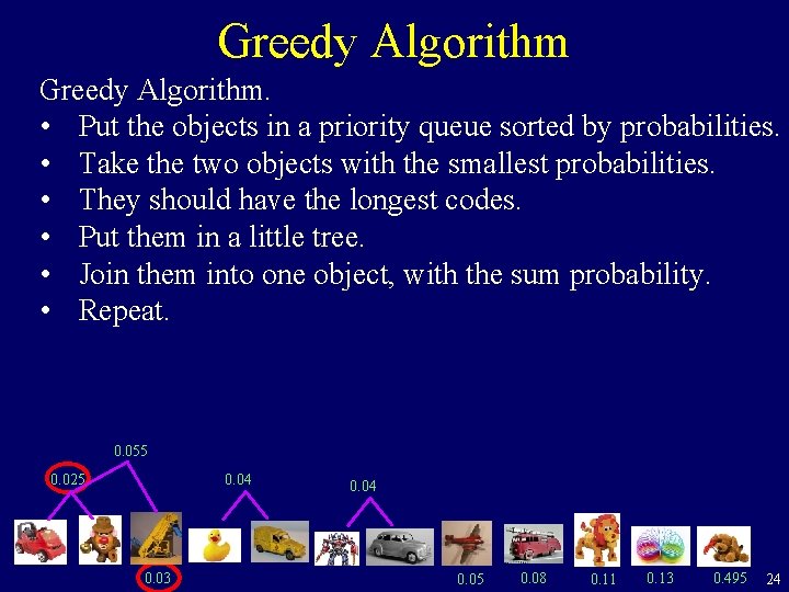
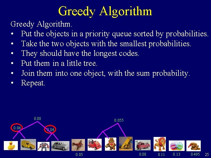
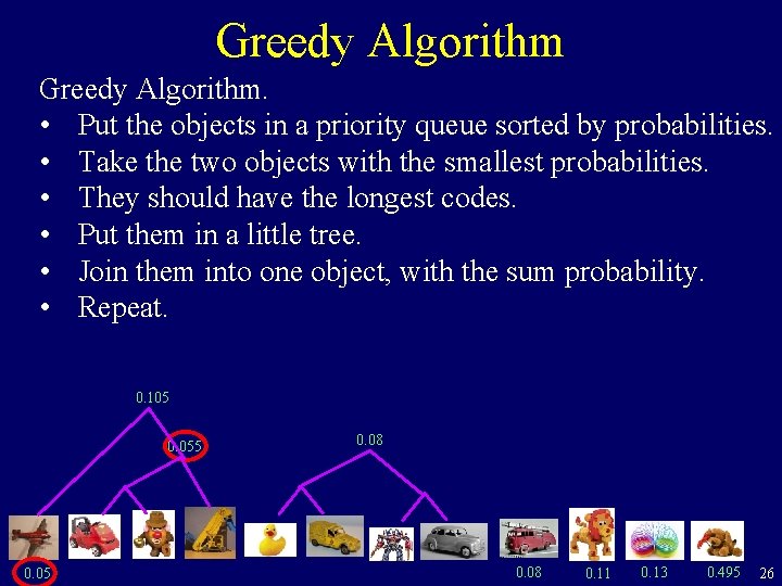
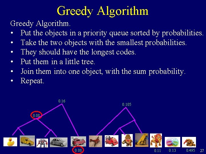
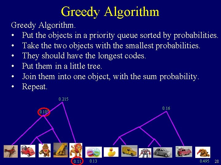
Communication & Entropy Greedy Algorithm. • Put the objects in a priority queue sorted by probabilities. • Take the two objects with the smallest probabilities. • They should have the longest codes. • Put them in a little tree. • Join them into one object, with the sum probability. • Repeat. 0. 025 0. 015 0. 02 0. 03 0. 05 0. 08 0. 11 0. 13 0. 495 8

Communication & Entropy Pi is the probability of the ith toy. Li is the length of the code for the ith toy. Claude Shannon (1948) Minimize: expected number of bits sent i pi Li Huffman’s algorithm says how to choose the code lengths Li. We want a nice equation for this number. Li Pi = 0. 01 0. 02 0. 08 0. 02 0. 031 0. 05 0. 11 0. 13 0. 495 9

Communication & Entropy Pi is the probability of the ith toy. Li is the length of the code for the ith toy. Claude Shannon (1948) 1/ 2 Pi = 0. 01 Minimize: expected number of bits sent i pi Li Subject to i 2 -Li = 1 1/ 0. 01 4 0. 02 1/ 0. 02 8 0. 08 1/ 0. 02 Li 16 0. 031 1/ 1/ 32 0. 05 0. 11 32 0. 13 0. 495 10

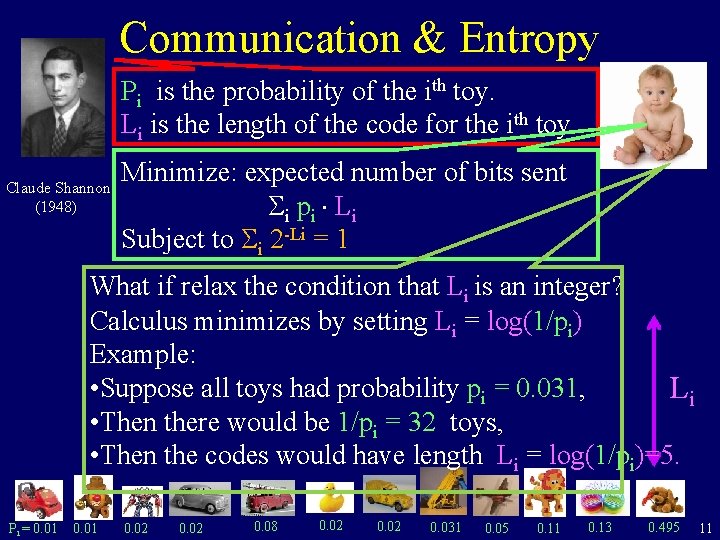
Communication & Entropy Pi is the probability of the ith toy. Li is the length of the code for the ith toy. Claude Shannon (1948) Minimize: expected number of bits sent i pi Li Subject to i 2 -Li = 1 What if relax the condition that Li is an integer? Calculus minimizes by setting Li = log(1/pi) Example: • Suppose all toys had probability pi = 0. 031, Li • Then there would be 1/pi = 32 toys, • Then the codes would have length Li = log(1/pi)=5. Pi = 0. 01 0. 02 0. 08 0. 02 0. 031 0. 05 0. 11 0. 13 0. 495 11

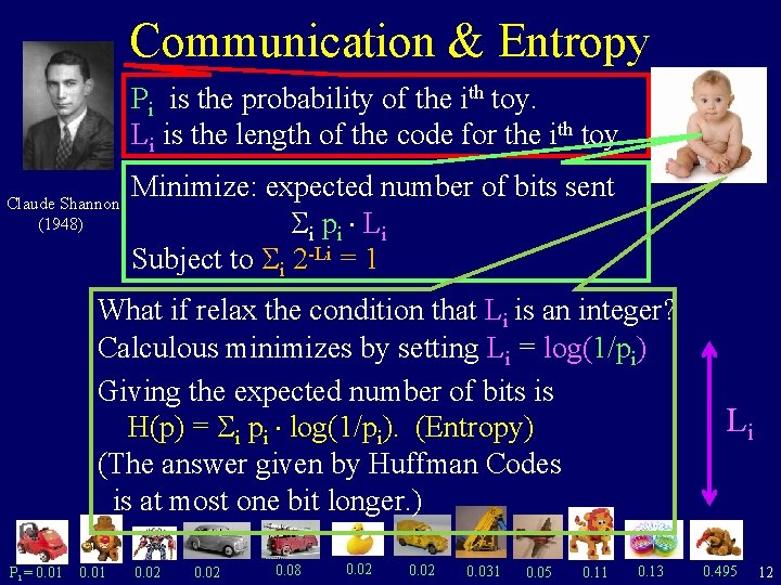
Communication & Entropy Pi is the probability of the ith toy. Li is the length of the code for the ith toy. Claude Shannon (1948) Minimize: expected number of bits sent i pi Li Subject to i 2 -Li = 1 What if relax the condition that Li is an integer? Calculous minimizes by setting Li = log(1/pi) Giving the expected number of bits is H(p) = i pi log(1/pi). (Entropy) (The answer given by Huffman Codes is at most one bit longer. ) Pi = 0. 01 0. 02 0. 08 0. 02 0. 031 0. 05 0. 11 0. 13 Li 0. 495 12

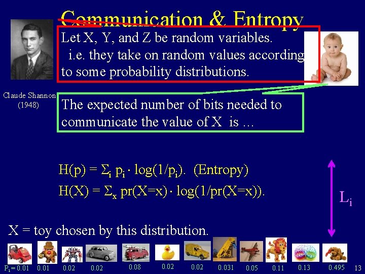
Communication & Entropy Let X, Y, and Z be random variables. i. e. they take on random values according to some probability distributions. Claude Shannon (1948) The expected number of bits needed to communicate the value of X is … H(p) = i pi log(1/pi). (Entropy) H(X) = x pr(X=x) log(1/pr(X=x)). Li X = toy chosen by this distribution. Pi = 0. 01 0. 02 0. 08 0. 02 0. 031 0. 05 0. 11 0. 13 0. 495 13

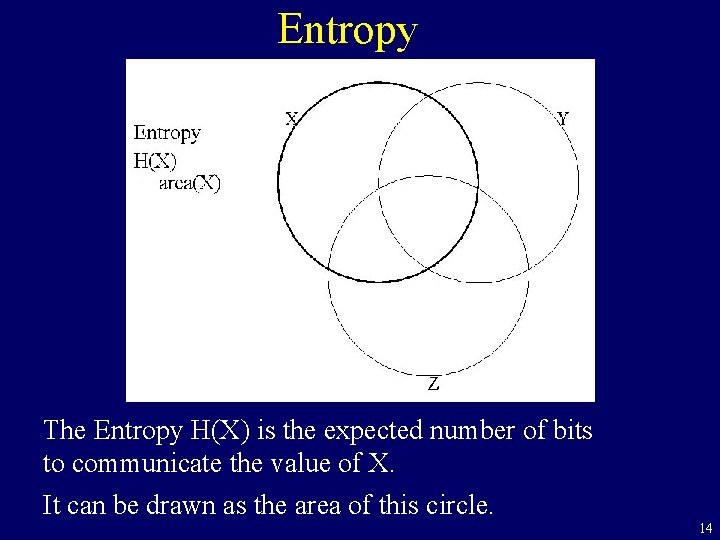
Entropy The Entropy H(X) is the expected number of bits to communicate the value of X. It can be drawn as the area of this circle. 14

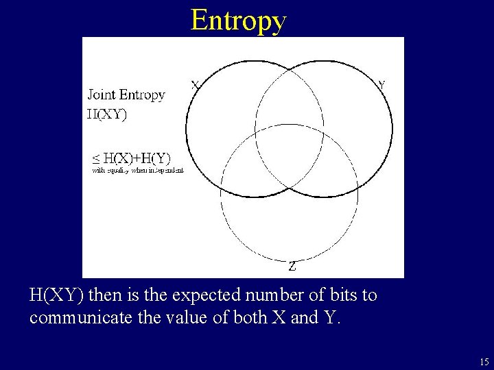
Entropy H(XY) then is the expected number of bits to communicate the value of both X and Y. 15

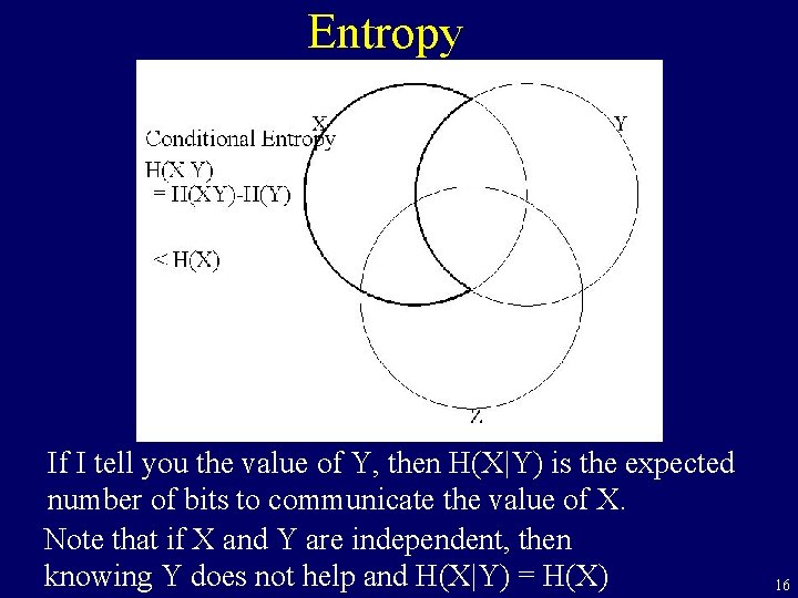
Entropy If I tell you the value of Y, then H(X|Y) is the expected number of bits to communicate the value of X. Note that if X and Y are independent, then knowing Y does not help and H(X|Y) = H(X) 16

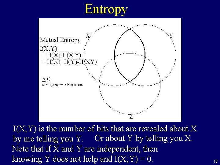
Entropy I(X; Y) is the number of bits that are revealed about X by me telling you Y. Or about Y by telling you X. Note that if X and Y are independent, then knowing Y does not help and I(X; Y) = 0. 17

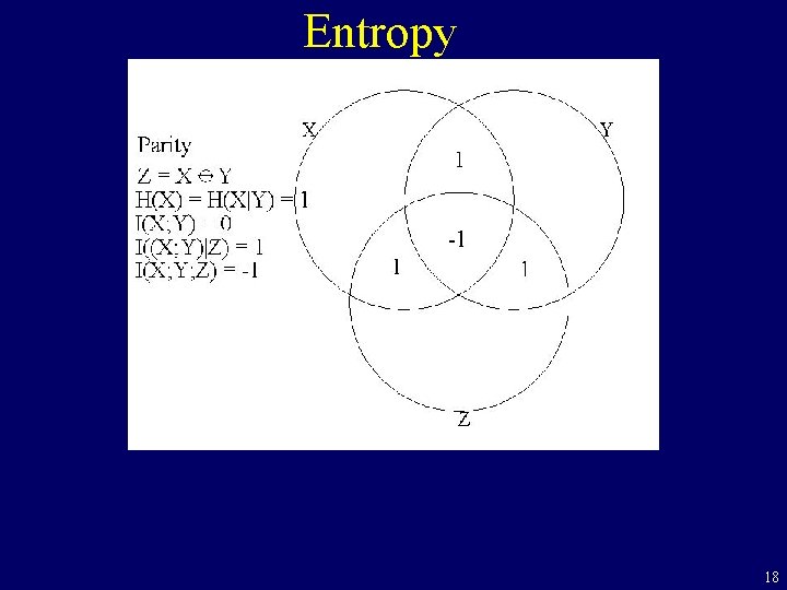
Entropy 18

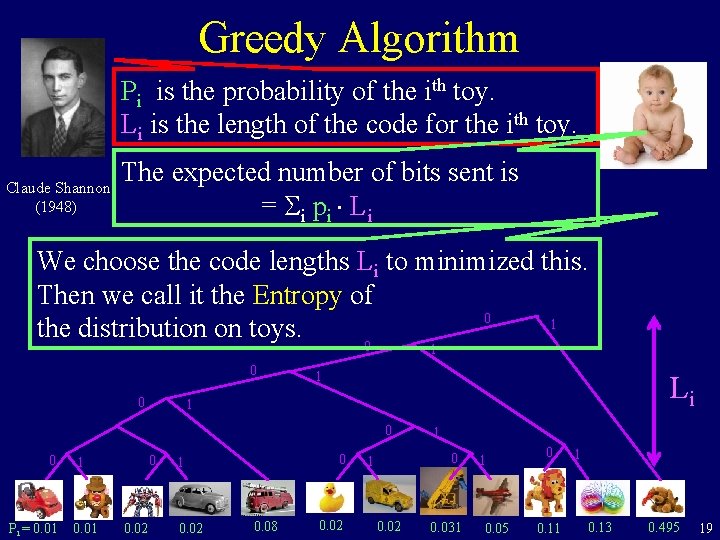
Greedy Algorithm Pi is the probability of the ith toy. Li is the length of the code for the ith toy. Claude Shannon (1948) The expected number of bits sent is = i pi Li We choose the code lengths Li to minimized this. Then we call it the Entropy of 0 1 the distribution on toys. 0 1 0 0 1 Li 1 0 0 Pi = 0. 01 0 1 0. 02 0. 08 0. 02 1 0. 02 0. 031 1 0. 05 0 0. 11 1 0. 13 0. 495 19

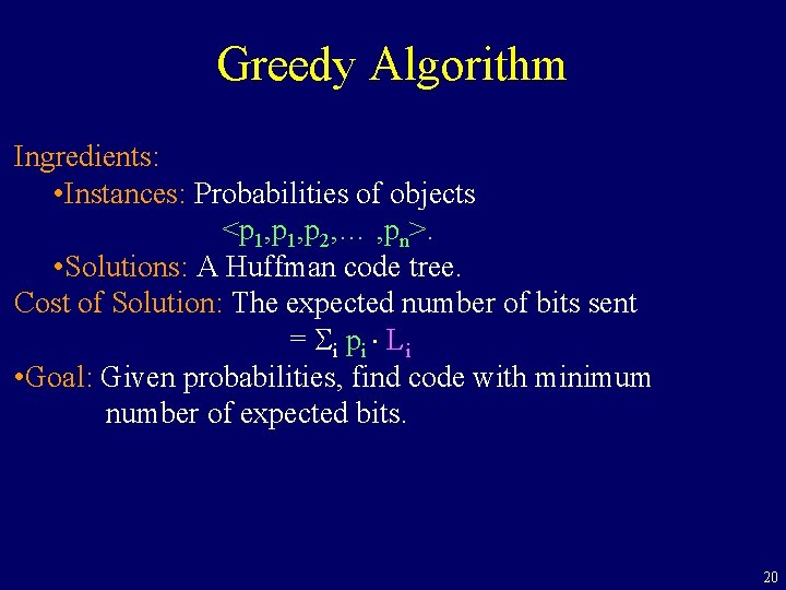
Greedy Algorithm Ingredients: • Instances: Probabilities of objects <p 1, p 2, … , pn>. • Solutions: A Huffman code tree. Cost of Solution: The expected number of bits sent = i pi Li • Goal: Given probabilities, find code with minimum number of expected bits. 20

Greedy Algorithm. • Put the objects in a priority queue sorted by probabilities. • Take the two objects with the smallest probabilities. • They should have the longest codes. • Put them in a little tree. • Join them into one object, with the sum probability. • Repeat. 0. 025 0. 015 0. 02 0. 03 0. 05 0. 08 0. 11 0. 13 0. 495 21

Greedy Algorithm. • Put the objects in a priority queue sorted by probabilities. • Take the two objects with the smallest probabilities. • They should have the longest codes. • Put them in a little tree. • Join them into one object, with the sum probability. • Repeat. 0. 025 0. 04 0. 02 0. 03 0. 05 0. 08 0. 11 0. 13 0. 495 22

Greedy Algorithm. • Put the objects in a priority queue sorted by probabilities. • Take the two objects with the smallest probabilities. • They should have the longest codes. • Put them in a little tree. • Join them into one object, with the sum probability. • Repeat. 0. 04 0. 025 0. 02 0. 04 0. 03 0. 05 0. 08 0. 11 0. 13 0. 495 23

Greedy Algorithm. • Put the objects in a priority queue sorted by probabilities. • Take the two objects with the smallest probabilities. • They should have the longest codes. • Put them in a little tree. • Join them into one object, with the sum probability. • Repeat. 0. 055 0. 04 0. 025 0. 03 0. 04 0. 05 0. 08 0. 11 0. 13 0. 495 24

Greedy Algorithm. • Put the objects in a priority queue sorted by probabilities. • Take the two objects with the smallest probabilities. • They should have the longest codes. • Put them in a little tree. • Join them into one object, with the sum probability. • Repeat. 0. 08 0. 04 0. 055 0. 04 0. 05 0. 08 0. 11 0. 13 0. 495 25

Greedy Algorithm. • Put the objects in a priority queue sorted by probabilities. • Take the two objects with the smallest probabilities. • They should have the longest codes. • Put them in a little tree. • Join them into one object, with the sum probability. • Repeat. 0. 105 0. 08 0. 11 0. 13 0. 495 26

Greedy Algorithm. • Put the objects in a priority queue sorted by probabilities. • Take the two objects with the smallest probabilities. • They should have the longest codes. • Put them in a little tree. • Join them into one object, with the sum probability. • Repeat. 0. 16 0. 105 0. 08 0. 11 0. 13 0. 495 27

Greedy Algorithm. • Put the objects in a priority queue sorted by probabilities. • Take the two objects with the smallest probabilities. • They should have the longest codes. • Put them in a little tree. • Join them into one object, with the sum probability. • Repeat. 0. 215 0. 16 0. 105 0. 11 0. 13 0. 495 28

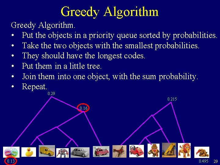
Greedy Algorithm. • Put the objects in a priority queue sorted by probabilities. • Take the two objects with the smallest probabilities. • They should have the longest codes. • Put them in a little tree. • Join them into one object, with the sum probability. • Repeat. 0. 29 0. 215 0. 16 0. 13 0. 495 29

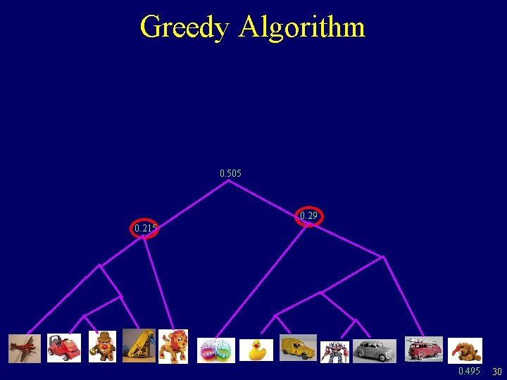
Greedy Algorithm 0. 505 0. 29 0. 215 0. 495 30

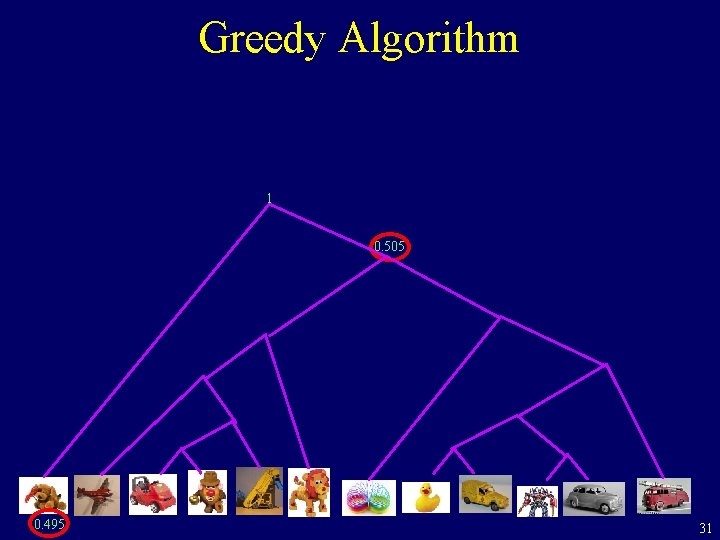
Greedy Algorithm 1 0. 505 0. 495 31

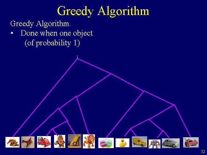
Greedy Algorithm. • Done when one object (of probability 1) 1 32

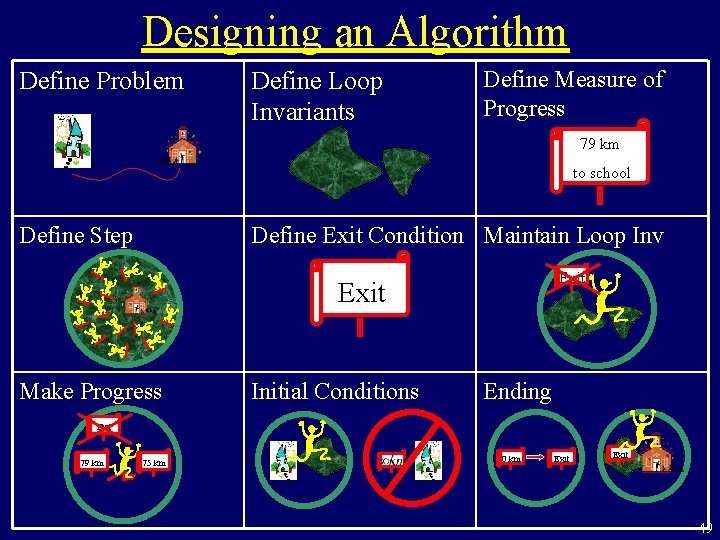
Designing an Algorithm Define Problem Define Loop Invariants Define Measure of Progress 79 km to school Define Step Define Exit Condition Maintain Loop Inv Exit Make Progress Initial Conditions Ending Exit 79 km 75 km 0 km Exit 33

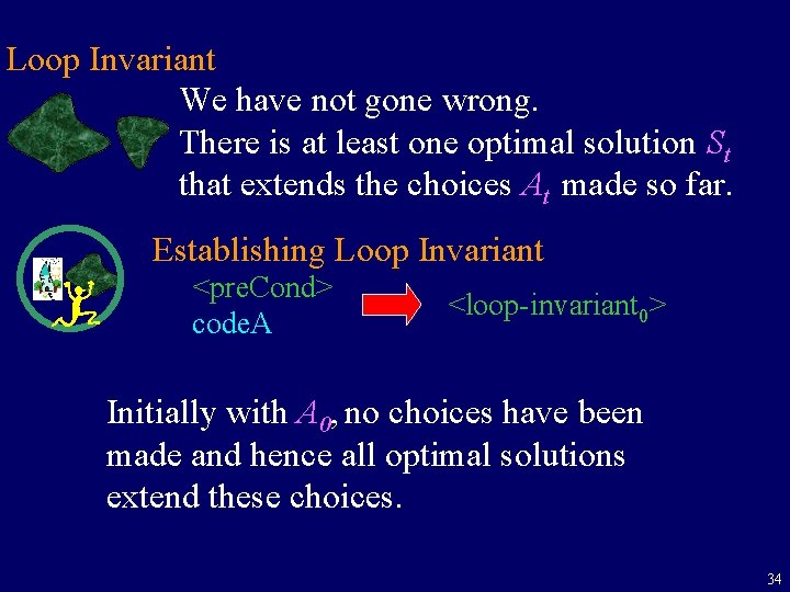
Loop Invariant We have not gone wrong. There is at least one optimal solution St that extends the choices At made so far. Establishing Loop Invariant <pre. Cond> code. A <loop-invariant 0> Initially with A 0, no choices have been made and hence all optimal solutions extend these choices. 34

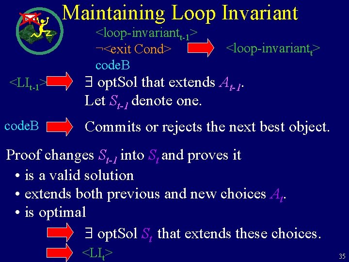
Exit Maintaining Loop Invariant <loop-invariantt-1> ¬<exit Cond> code. B <LIt-1> code. B <loop-invariantt> $ opt. Sol that extends At-1. Let St-1 denote one. Commits or rejects the next best object. Proof changes St-1 into St and proves it • is a valid solution • extends both previous and new choices At. • is optimal $ opt. Sol St that extends these choices. <LIt> 35

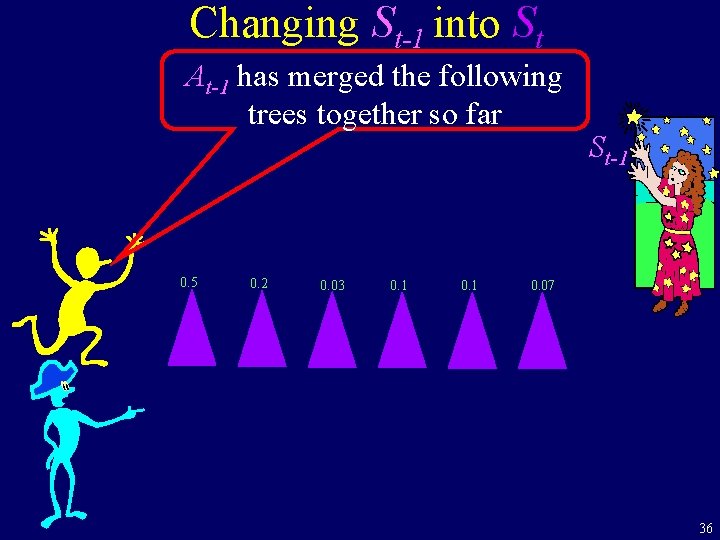
Changing St-1 into St At-1 has merged the following trees together so far 0. 5 0. 2 0. 03 0. 1 St-1 0. 07 36

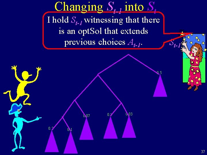
Changing St-1 into St I hold St-1 witnessing that there is an opt. Sol that extends previous choices At-1. St-1 0. 5 0. 07 0. 2 0. 1 0. 03 0. 1 37

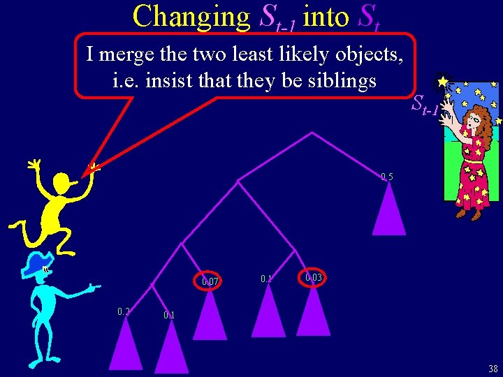
Changing St-1 into St I merge the two least likely objects, i. e. insist that they be siblings St-1 0. 5 0. 07 0. 2 0. 1 0. 03 0. 1 38

Changing St-1 into St I instruct how to change St-1 into St so that it extends previous & new choice. St-1 0. 5 0. 07 0. 2 0. 1 0. 03 0. 1 39

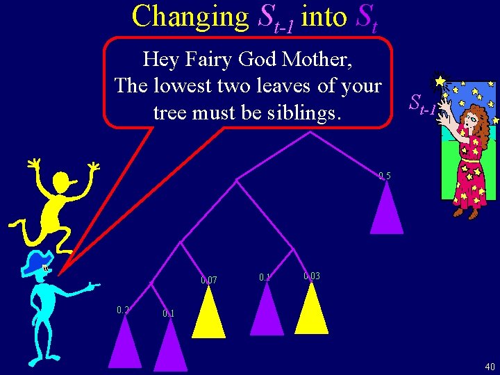
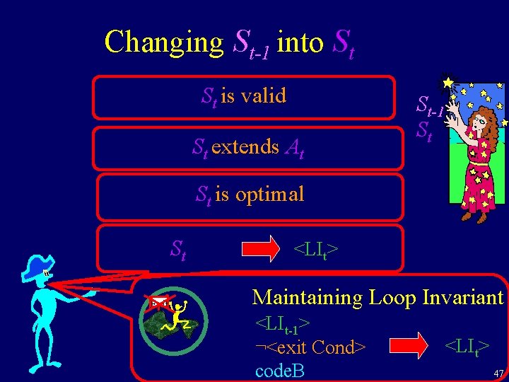
Changing St-1 into St Hey Fairy God Mother, The lowest two leaves of your tree must be siblings. St-1 0. 5 0. 07 0. 2 0. 1 0. 03 0. 1 40

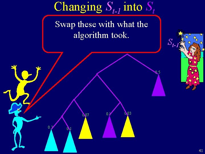
Changing St-1 into St Swap these with what the algorithm took. St-1 0. 5 0. 07 0. 2 0. 1 0. 03 0. 1 41

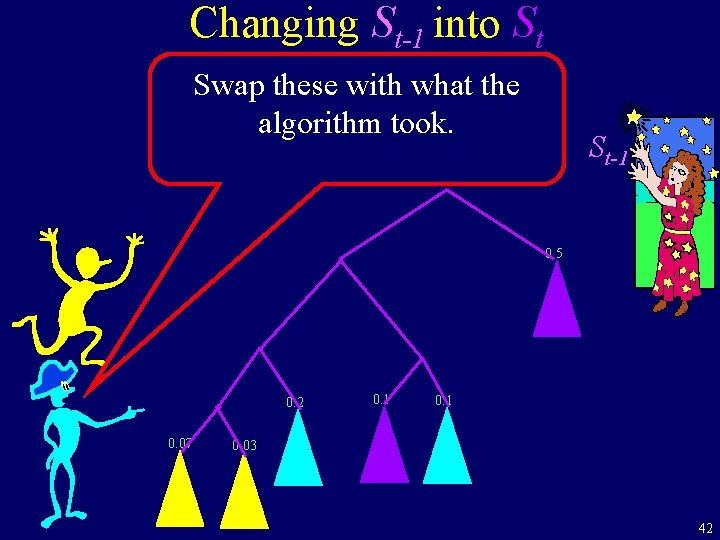
Changing St-1 into St Swap these with what the algorithm took. St-1 0. 5 0. 2 0. 07 0. 1 0. 03 42

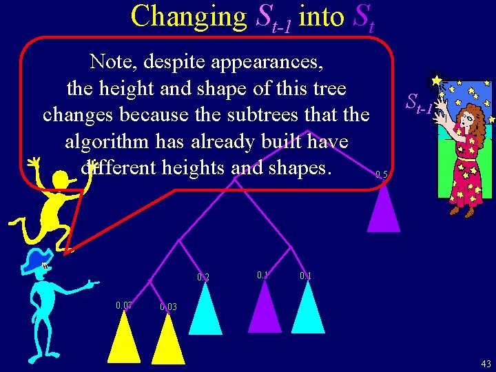
Changing St-1 into St Note, despite appearances, the height and shape of this tree St-1 changes because the subtrees that the algorithm has already built have different heights and shapes. 0. 5 0. 2 0. 07 0. 1 0. 03 43

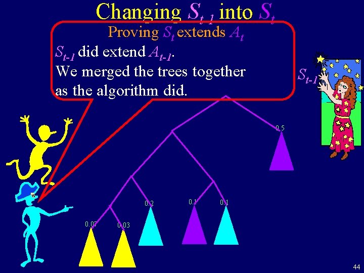
Changing St-1 into St Proving St extends At St-1 did extend At-1. We merged the trees together as the algorithm did. St-1 0. 5 0. 2 0. 07 0. 1 0. 03 44

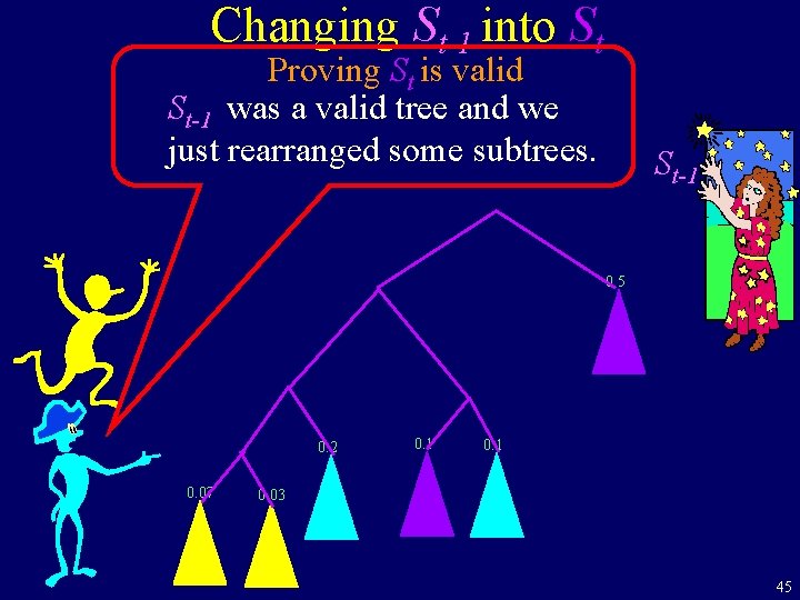
Changing St-1 into St Proving St is valid St-1 was a valid tree and we just rearranged some subtrees. St-1 0. 5 0. 2 0. 07 0. 1 0. 03 45

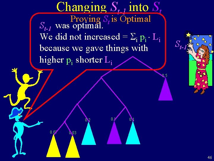
Changing St-1 into St Proving St is Optimal St-1 was optimal. We did not increased = i pi Li because we gave things with higher pi shorter Li St-1 0. 5 0. 2 0. 07 0. 1 0. 03 46

Changing St-1 into St St is valid St extends At St-1 St St is optimal St Exit <LIt> Maintaining Loop Invariant <LIt-1> ¬<exit Cond> code. B <LIt> 47

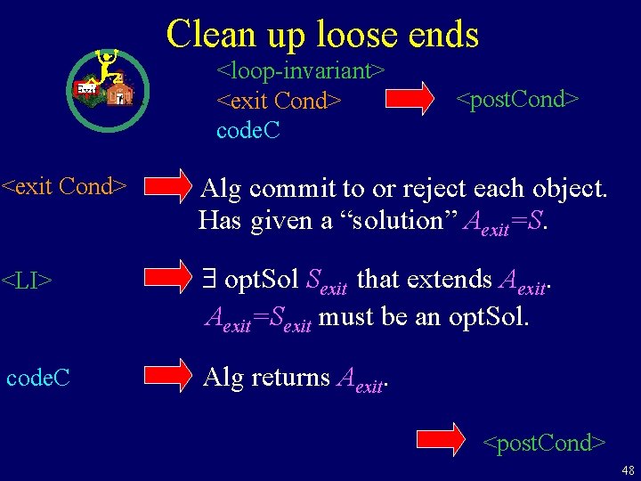
Clean up loose ends Exit <loop-invariant> <exit Cond> code. C <post. Cond> <exit Cond> Alg commit to or reject each object. Has given a “solution” Aexit=S. <LI> $ opt. Sol Sexit that extends Aexit=Sexit must be an opt. Sol. code. C Alg returns Aexit. <post. Cond> 48

Designing an Algorithm Define Problem Define Loop Invariants Define Measure of Progress 79 km to school Define Step Define Exit Condition Maintain Loop Inv Exit Make Progress Initial Conditions Ending Exit 79 km 75 km 0 km Exit 49