Communication Cost in Parallel Query Processing Dan Suciu

This Talk • How much communication is needed to compute a query Q on

Massively Parallel Communication Model (MPC) Extends BSP [Valiant] Input (size=m) Input data = size

Example: Join(x, y, z) = R(x, y), S(y, z) S |R|=|S|=m R x y

Speedup Speed A load of L = m/p corresponds to linear speedup # processors

Outline • The MPC Model • The Algorithm • Skew matters • Statistics matter

Overview Computes a full conjunctive query in one round of communication, by partial replication.

The Triangle Query T • Input: three tables R(X, Y), S(Y, Z), T(Z, X)

|R| = |S| = |T| = m tuples Trianges(x, y, z) = R(x, y),

Trianges(x, y, z) = R(x, y), S(y, z), T(z, x) |R| = |S| =

Hper. Cube Algorithm for Full CQ • Write: p = p 1 * p

Computing Shares p 1, p 2, …, pk Suppose all relations have the same

Fractional Vertex Cover Hyper-graph: nodes x 1, x 2 …, hyper-edges S 1, S

L = m / p 1/τ* Examples Integral vertex cover t* = 2 Triangles(x,

Lessons So Far • MPC model: cost = communication load + rounds • Hyper.

Skew Matters • If the database is skewed, the query becomes provably harder. We

Skew Matters 0 • Join(x, y, z) = R(x, y), S(y, z) 1 0

All You Need to Know About Skew Hash-partition a bag of m data values

Atserias, Grohe, Marx’ 13 The AGM Inequality Suppose all relations have the same size

The AGM Inequality Suppose all relations have the same size m Fact. Any MPC

Lessons so Far • Skew affects communication dramatically – w/o skew: L = m

Statistics • So far: all relations have same size m • In reality, we

Statistics for Cartesian Product 2 -way product Q(x, y) = S 1(x) × S

Fractional Edge Packing Hyper-graph: nodes x 1, x 2 …, hyper-edges S 1, S

Statistics for a Query Q Relations data-sizes= m 1, m 2, … Then, for

Example ½ Trianges(x, y, z) = R(x, y), S(y, z), T(z, x) ½ ½

Discussion Speedup Fact 1 L = [geometric-mean of m 1, m 2, . .

Coping with Skew Definition A value c is a “heavy hitter” for xi in

Coping with Skew What we know today: • Join(x, y, z) = R(x, y),

Multiple Rounds What we would like: • Reduce load below m/p 1/τ* – ACQ

More Resources • Extended slides, exercises, open problems: Ph. D Open Warsaw, March 2015

Slides: 50

Download presentation

Communication Cost in Parallel Query Processing Dan Suciu University of Washington Joint work with Paul Beame, Paris Koutris and the Myria Team Beyond MR - March 2015 1

This Talk • How much communication is needed to compute a query Q on p servers?

Massively Parallel Communication Model (MPC) Extends BSP [Valiant] Input (size=m) Input data = size m O(m/p) Server 1 Number of servers = p . . O(m/p) Server p

Massively Parallel Communication Model (MPC) Extends BSP [Valiant] Input (size=m) Input data = size m O(m/p) Server 1 Number of servers = p One round = Compute & communicate . . ≤L Server 1 ≤L Round 1. . Server 1 Server p ≤L Round 2 ≤L Algorithm = Several rounds O(m/p) Server p . . ≤L Server p ≤L Round 3 . .

Massively Parallel Communication Model (MPC) Extends BSP [Valiant] Input (size=m) Input data = size m O(m/p) Server 1 Number of servers = p One round = Compute & communicate . . ≤L Server 1 ≤L Round 1. . Server 1 Max communication load / round / server = L Server p ≤L Round 2 ≤L Algorithm = Several rounds O(m/p) Server p . . ≤L Server p ≤L Round 3 . .

Massively Parallel Communication Model (MPC) Extends BSP [Valiant] Input (size=m) Input data = size m O(m/p) Server 1 Number of servers = p . . ≤L One round = Compute & communicate Server 1 ≤L Round 1. . Server 1 Max communication load / round / server = L Server p ≤L Round 2 ≤L Algorithm = Several rounds O(m/p) Server p . . ≤L Server p ≤L Round 3 . . Cost: Ideal Load L L = m/p Rounds r 1 Practical ε∈(0, 1) L = m/p 1 -ε O(1) Naïve 1 L=m 1 Naïve 2 L = m/p p

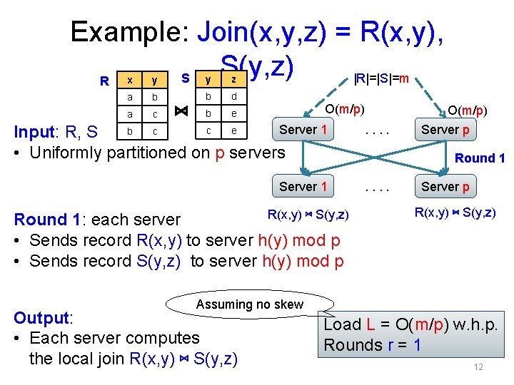
Example: Join(x, y, z) = R(x, y), S(y, z) S |R|=|S|=m R x y y z a b b d a c b e ⋈ O(m/p) Server 1 c e b c Input: R, S • Uniformly partitioned on p servers . . Server 1 . . R(x, y) ⋈ S(y, z) Round 1: each server • Sends record R(x, y) to server h(y) mod p • Sends record S(y, z) to server h(y) mod p O(m/p) Server p Round 1 Server p R(x, y) ⋈ S(y, z) Assuming no skew Output: • Each server computes the local join R(x, y) ⋈ S(y, z) Load L = O(m/p) w. h. p. Rounds r = 1 12

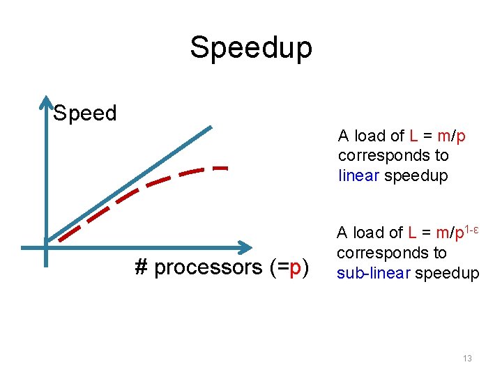
Speedup Speed A load of L = m/p corresponds to linear speedup # processors (=p) A load of L = m/p 1 -ε corresponds to sub-linear speedup 13

Outline • The MPC Model • The Algorithm • Skew matters • Statistics matter • Extensions and Open Problems 14

Overview Computes a full conjunctive query in one round of communication, by partial replication. • The tradeoff was discussed [Ganguli’ 92] • Shares Algorithm: [Afrati&Ullman’ 10] – For Map. Reduce • Hyper. Cube Algorithm [Beame’ 13, ’ 14] – Same as in Shares – But different optimization/analysis 15

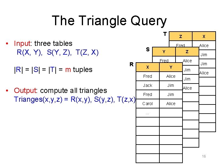
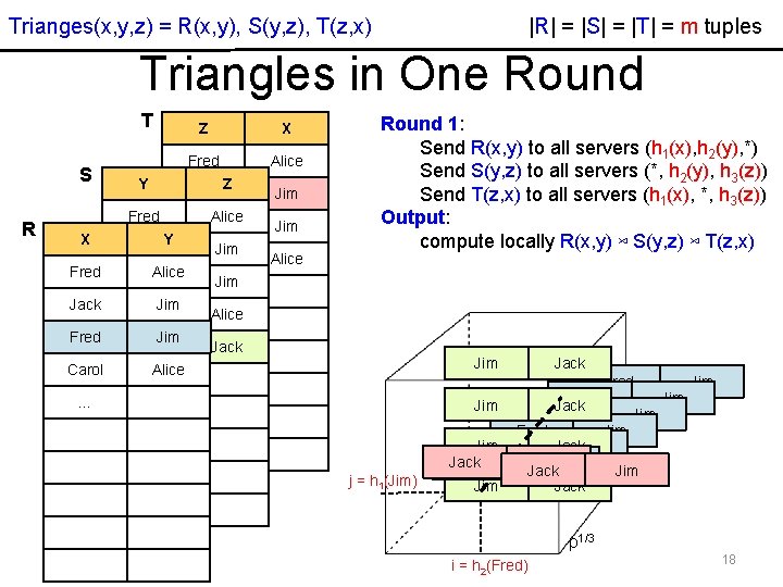
The Triangle Query T • Input: three tables R(X, Y), S(Y, Z), T(Z, X) |R| = |S| = |T| = m tuples S R X Fred • Output: compute all triangles Trianges(x, y, z) = R(x, y), S(y, z), T(z, x) Jack Fred Carol Y Z X Fred Alice Z Jack Fred Alice Fred Y Jack Jim Carol Alice Fred Jim … Jim Carol Alice Jim … Alice Jim Alice … 16

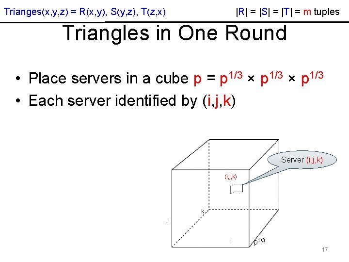
|R| = |S| = |T| = m tuples Trianges(x, y, z) = R(x, y), S(y, z), T(z, x) Triangles in One Round • Place servers in a cube p = p 1/3 × p 1/3 • Each server identified by (i, j, k) Server (i, j, k) k j i p 1/3 17

|R| = |S| = |T| = m tuples Trianges(x, y, z) = R(x, y), S(y, z), T(z, x) Triangles in One Round T S R X Fred Jack Fred Carol Y Z X Fred Alice Z Jack Fred Alice Fred Y Jack Jim Carol Alice Fred Jim … Jim Carol Alice Jim Jack Alice Jim Alice Round 1: Send R(x, y) to all servers (h 1(x), h 2(y), *) Send S(y, z) to all servers (*, h 2(y), h 3(z)) Send T(z, x) to all servers (h 1(x), *, h 3(z)) Output: compute locally R(x, y) ⋈ S(y, z) ⋈ T(z, x) Jim Jack Fred Jim Jim Jack Fred Jim Jack Jim Jack (i, j, k) … j = h 1(Jim) p 1/3 i = h 2(Fred) 18

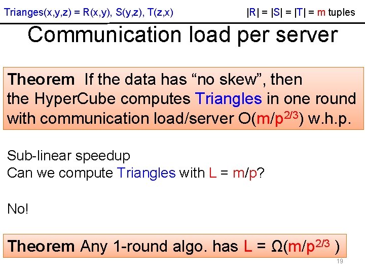
Trianges(x, y, z) = R(x, y), S(y, z), T(z, x) |R| = |S| = |T| = m tuples Communication load per server Theorem If the data has “no skew”, then the Hyper. Cube computes Triangles in one round with communication load/server O(m/p 2/3) w. h. p. Sub-linear speedup Can we compute Triangles with L = m/p? No! Theorem Any 1 -round algo. has L = Ω(m/p 2/3 ) 19

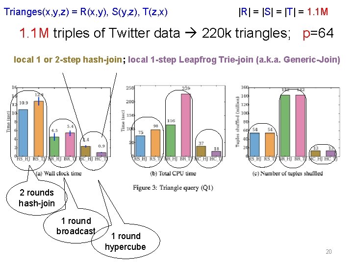
Trianges(x, y, z) = R(x, y), S(y, z), T(z, x) |R| = |S| = |T| = 1. 1 M triples of Twitter data 220 k triangles; p=64 local 1 or 2 -step hash-join; local 1 -step Leapfrog Trie-join (a. k. a. Generic-Join) 2 rounds hash-join 1 round broadcast 1 round hypercube 20

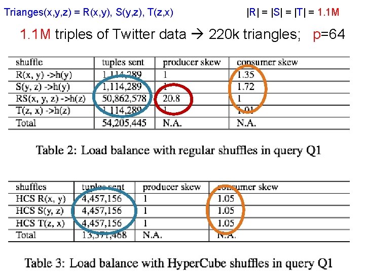
Trianges(x, y, z) = R(x, y), S(y, z), T(z, x) |R| = |S| = |T| = 1. 1 M triples of Twitter data 220 k triangles; p=64

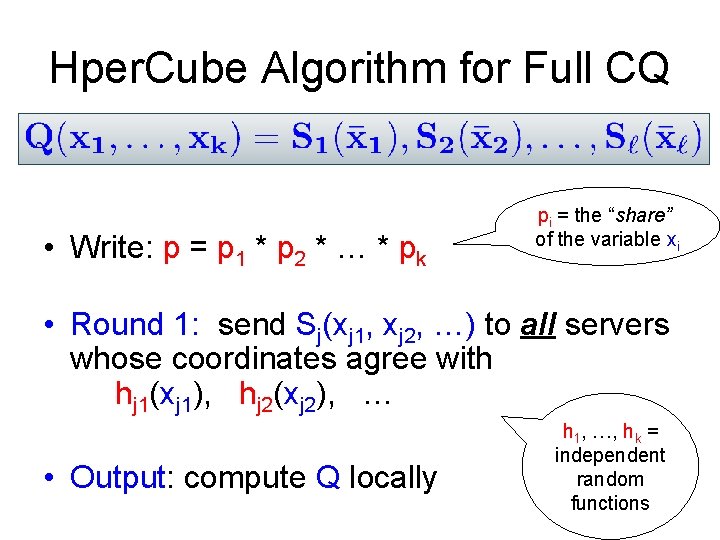
Hper. Cube Algorithm for Full CQ • Write: p = p 1 * p 2 * … * pk pi = the “share” of the variable xi • Round 1: send Sj(xj 1, xj 2, …) to all servers whose coordinates agree with hj 1(xj 1), hj 2(xj 2), … • Output: compute Q locally h 1, …, hk = independent random functions

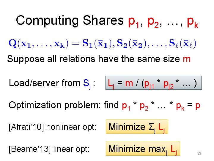
Computing Shares p 1, p 2, …, pk Suppose all relations have the same size m Load/server from Sj : Lj = m / (pj 1 * pj 2 * … ) Optimization problem: find p 1 * p 2 * … * pk = p [Afrati’ 10] nonlinear opt: Minimize Σj Lj [Beame’ 13] linear opt: Minimize maxj Lj 23

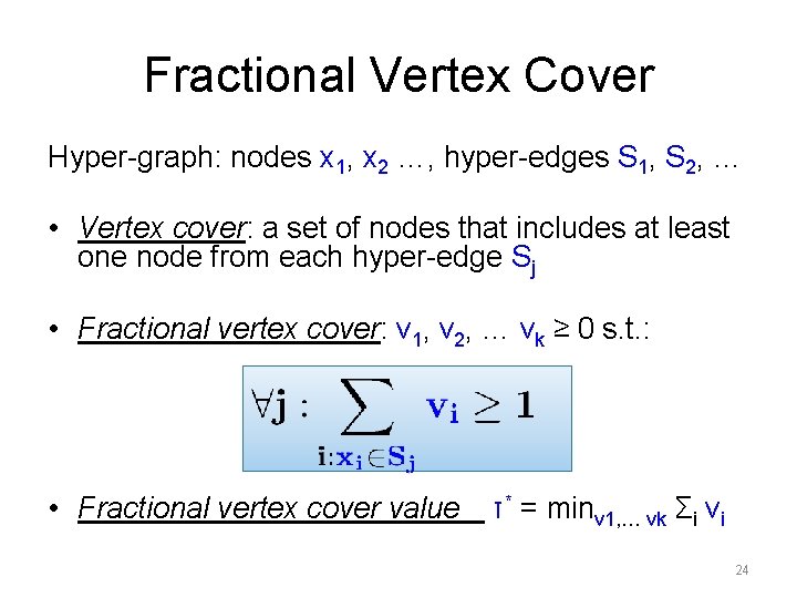
Fractional Vertex Cover Hyper-graph: nodes x 1, x 2 …, hyper-edges S 1, S 2, … • Vertex cover: a set of nodes that includes at least one node from each hyper-edge Sj • Fractional vertex cover: v 1, v 2, … vk ≥ 0 s. t. : • Fractional vertex cover value τ* = minv 1, … vk Σi vi 24

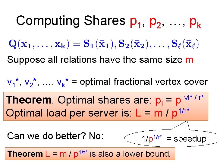
Computing Shares p 1, p 2, …, pk Suppose all relations have the same size m v 1*, v 2*, …, vk* = optimal fractional vertex cover Theorem. Optimal shares are: pi = p vi* / τ* Optimal load per server is: L = m / p 1/τ* Can we do better? No: 1/p 1/τ* = speedup Theorem L = m / p 1/τ* is also a lower bound.

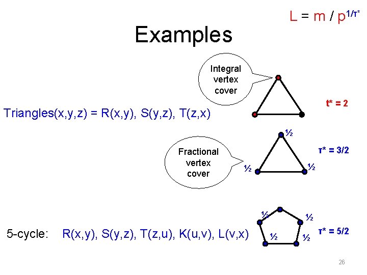
L = m / p 1/τ* Examples Integral vertex cover t* = 2 Triangles(x, y, z) = R(x, y), S(y, z), T(z, x) ½ Fractional vertex cover τ* = 3/2 ½ ½ ½ 5 -cycle: R(x, y), S(y, z), T(z, u), K(u, v), L(v, x) ½ ½ ½ τ* = 5/2 26

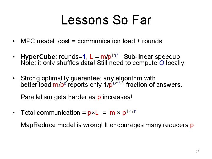
Lessons So Far • MPC model: cost = communication load + rounds • Hyper. Cube: rounds=1, L = m/p 1/τ* Sub-linear speedup Note: it only shuffles data! Still need to compute Q locally. • Strong optimality guarantee: any algorithm with better load m/ps reports only 1/ps×τ*-1 fraction of answers. Parallelism gets harder as p increases! • Total communication = p×L = m × p 1 -1/τ* Map. Reduce model is wrong! It encourages many reducers p 27

Outline • The MPC Model • The Algorithm • Skew matters • Statistics matter • Extensions and Open Problems 28

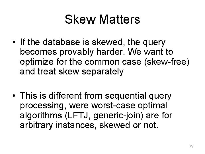
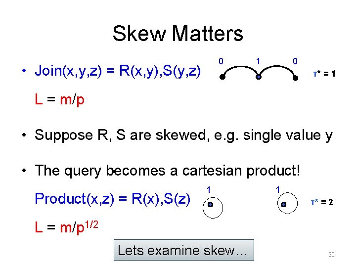
Skew Matters • If the database is skewed, the query becomes provably harder. We want to optimize for the common case (skew-free) and treat skew separately • This is different from sequential query processing, were worst-case optimal algorithms (LFTJ, generic-join) are for arbitrary instances, skewed or not. 29

Skew Matters 0 • Join(x, y, z) = R(x, y), S(y, z) 1 0 τ* = 1 L = m/p • Suppose R, S are skewed, e. g. single value y • The query becomes a cartesian product! Product(x, z) = R(x), S(z) 1 1 τ* = 2 L = m/p 1/2 Lets examine skew… 30

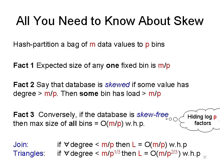
All You Need to Know About Skew Hash-partition a bag of m data values to p bins Fact 1 Expected size of any one fixed bin is m/p Fact 2 Say that database is skewed if some value has degree > m/p. Then some bin has load > m/p Fact 3 Conversely, if the database is skew-free then max size of all bins = O(m/p) w. h. p. Join: Triangles: Hiding log p factors if ∀degree < m/p then L = O(m/p) w. h. p if ∀degree < m/p 1/3 then L = O(m/p 2/3 ) w. h. p 31

Atserias, Grohe, Marx’ 13 The AGM Inequality Suppose all relations have the same size m Theorem. [AGM] Let u 1, u 2, …, ul be an optimal fractional edge cover, and ρ* = u 1+u 2+ … +ul Then: |Q| ≤ mρ* 32

The AGM Inequality Suppose all relations have the same size m Fact. Any MPC algorithm using r rounds and load/server L satisfies r×L ≥ m / p 1/ρ* Proof. • Tightness of AGM: there exists db s. t. |Q| = mρ* • AGM: one server reports only (r×L)ρ* answers • All p servers report only p×(r×L)ρ* answers 33 ? WAIT: we computed Join with L = m / p now we say L ≥ m / p 1/2

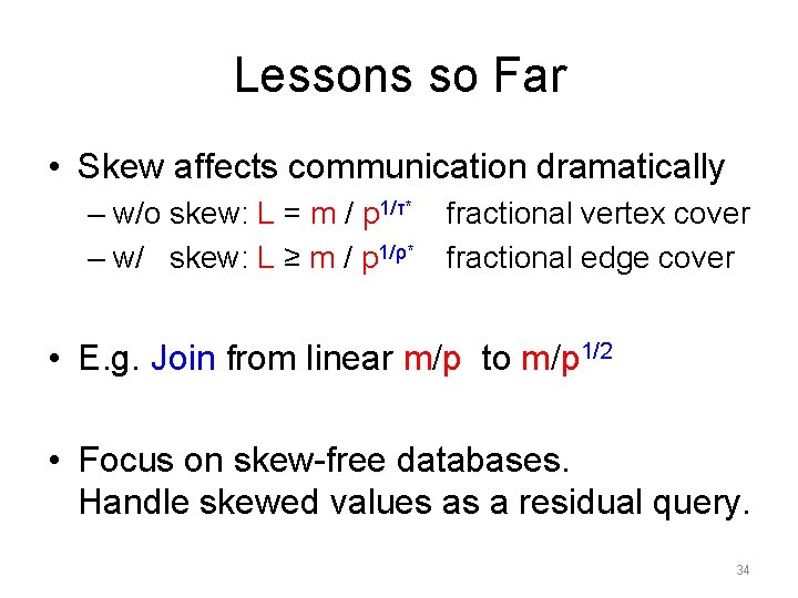
Lessons so Far • Skew affects communication dramatically – w/o skew: L = m / p 1/τ* – w/ skew: L ≥ m / p 1/ρ* fractional vertex cover fractional edge cover • E. g. Join from linear m/p to m/p 1/2 • Focus on skew-free databases. Handle skewed values as a residual query. 34

Outline • The MPC Model • The Algorithm • Skew matters • Statistics matter • Extensions and Open Problems 35

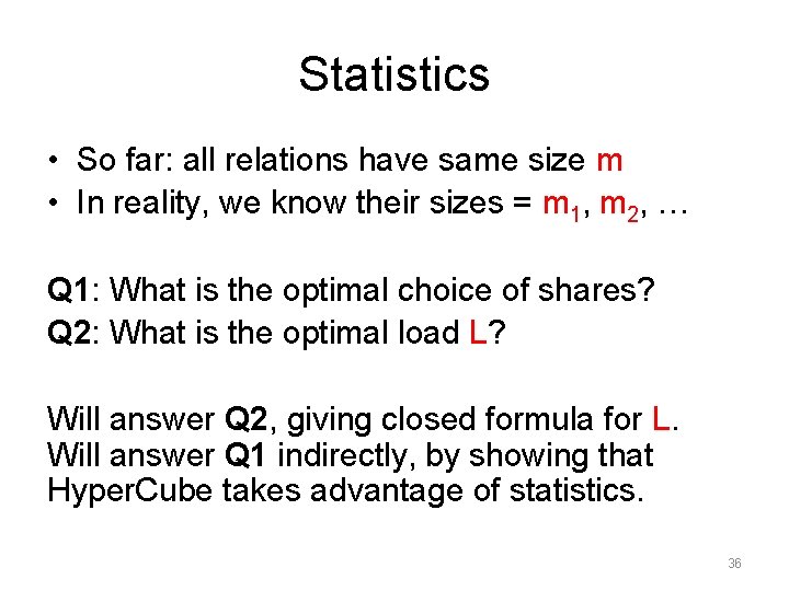
Statistics • So far: all relations have same size m • In reality, we know their sizes = m 1, m 2, … Q 1: What is the optimal choice of shares? Q 2: What is the optimal load L? Will answer Q 2, giving closed formula for L. Will answer Q 1 indirectly, by showing that Hyper. Cube takes advantage of statistics. 36

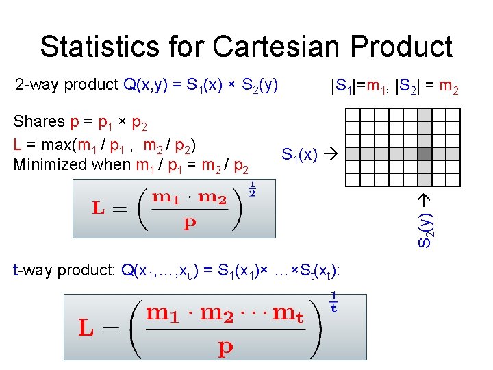
Statistics for Cartesian Product 2 -way product Q(x, y) = S 1(x) × S 2(y) S 1(x) S 2(y) Shares p = p 1 × p 2 L = max(m 1 / p 1 , m 2 / p 2) Minimized when m 1 / p 1 = m 2 / p 2 |S 1|=m 1, |S 2| = m 2 t-way product: Q(x 1, …, xu) = S 1(x 1)× …×St(xt):

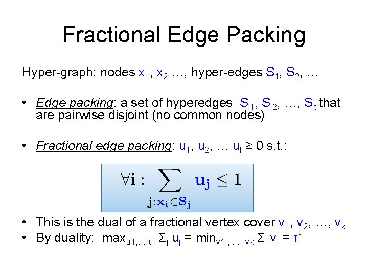
Fractional Edge Packing Hyper-graph: nodes x 1, x 2 …, hyper-edges S 1, S 2, … • Edge packing: a set of hyperedges Sj 1, Sj 2, …, Sjt that are pairwise disjoint (no common nodes) • Fractional edge packing: u 1, u 2, … ul ≥ 0 s. t. : • This is the dual of a fractional vertex cover v 1, v 2, …, vk • By duality: maxu 1, … ul Σj uj = minv 1, , …, vk Σi vi = τ*

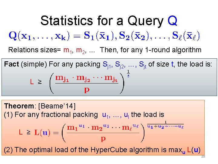
Statistics for a Query Q Relations sizes= m 1, m 2, … Then, for any 1 -round algorithm Fact (simple) For any packing Sj 1, Sj 2, …, Sjt of size t, the load is: L ≥ Theorem: [Beame’ 14] (1) For any fractional packing u 1, …, ul the load is L ≥ (2) The optimal load of the Hyper. Cube algorithm is maxu L(u) 39

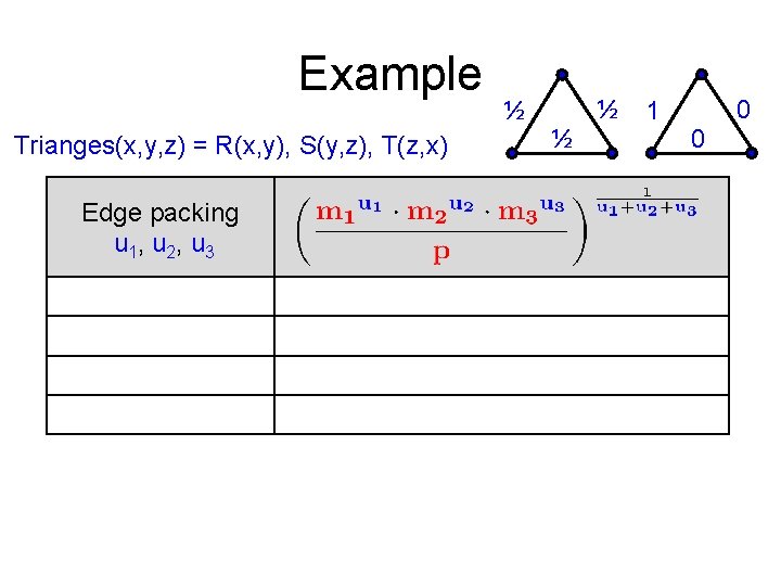
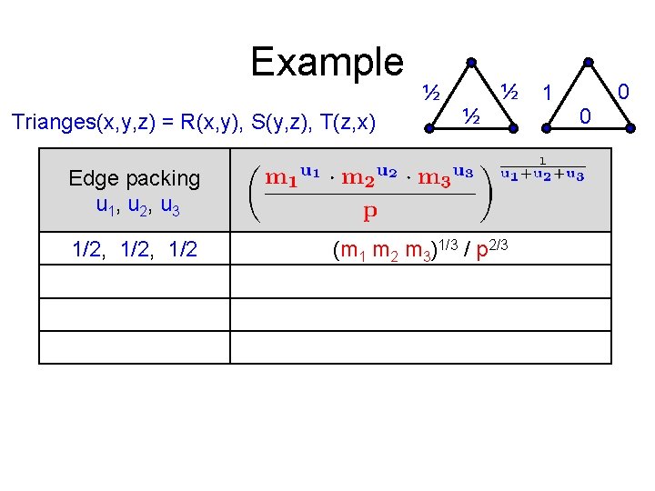
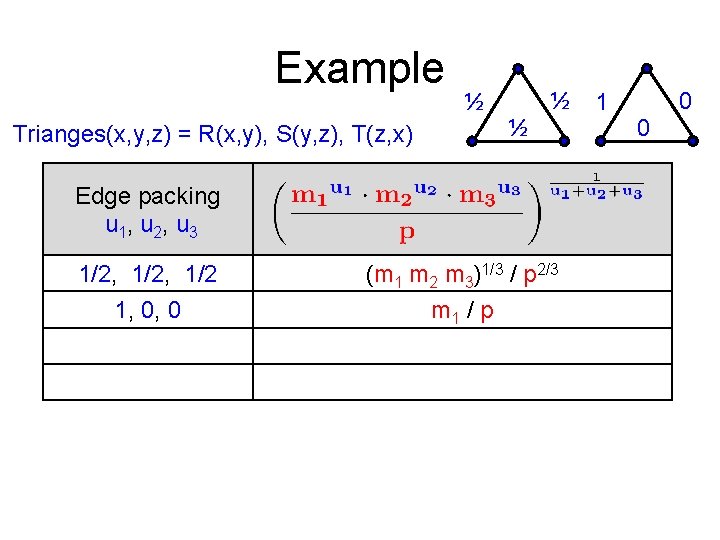
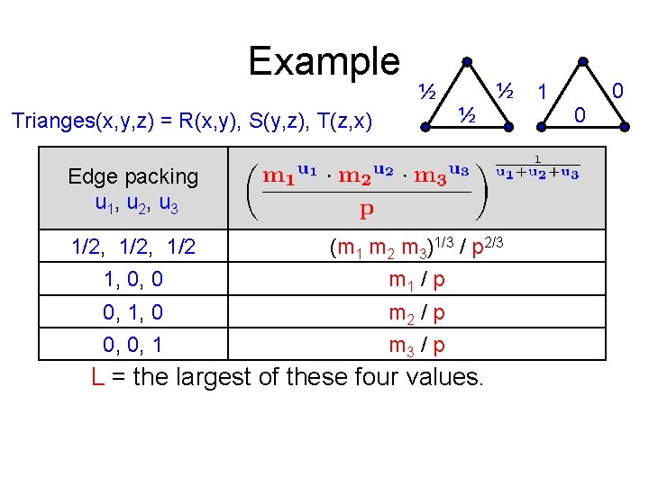
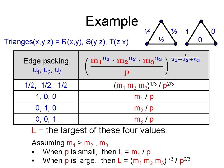
Example ½ Trianges(x, y, z) = R(x, y), S(y, z), T(z, x) ½ ½ Edge packing u 1, u 2, u 3 1/2, 1/2 (m 1 m 2 m 3)1/3 / p 2/3 1, 0, 0 m 1 / p 0, 1, 0 m 2 / p 0, 0, 1 m 3 / p 1 0 0

Example ½ Trianges(x, y, z) = R(x, y), S(y, z), T(z, x) ½ ½ Edge packing u 1, u 2, u 3 1/2, 1/2 (m 1 m 2 m 3)1/3 / p 2/3 1, 0, 0 m 1 / p 0, 1, 0 m 2 / p 0, 0, 1 m 3 / p L = the largest of these four values. 1 0 0

Example ½ Trianges(x, y, z) = R(x, y), S(y, z), T(z, x) ½ ½ 1 Edge packing u 1, u 2, u 3 1/2, 1/2 (m 1 m 2 m 3)1/3 / p 2/3 1, 0, 0 m 1 / p 0, 1, 0 m 2 / p 0, 0, 1 m 3 / p L = the largest of these four values. Assuming m 1 > m 2 , m 3 • When p is small, then L = m 1 / p. • When p is large, then L = (m 1 m 2 m 3)1/3 / p 2/3 0 0

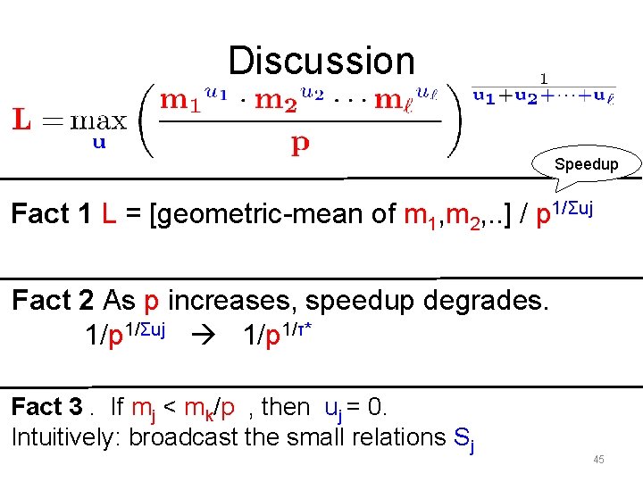
Discussion Speedup Fact 1 L = [geometric-mean of m 1, m 2, . . ] / p 1/Σuj Fact 2 As p increases, speedup degrades. 1/p 1/Σuj 1/p 1/τ* Fact 3. If mj < mk/p , then uj = 0. Intuitively: broadcast the small relations Sj 45

Outline • The MPC Model • The Algorithm • Skew matters • Statistics matter • Extensions and Open Problems 46

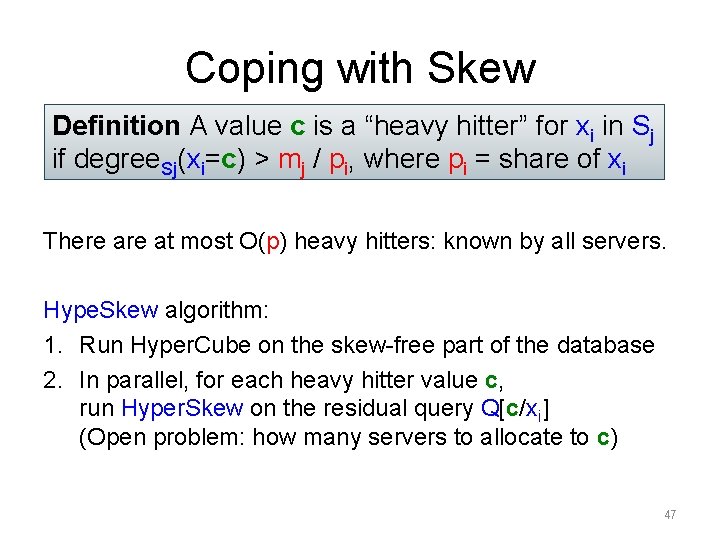
Coping with Skew Definition A value c is a “heavy hitter” for xi in Sj if degree. Sj(xi=c) > mj / pi, where pi = share of xi There at most O(p) heavy hitters: known by all servers. Hype. Skew algorithm: 1. Run Hyper. Cube on the skew-free part of the database 2. In parallel, for each heavy hitter value c, run Hyper. Skew on the residual query Q[c/xi] (Open problem: how many servers to allocate to c) 47

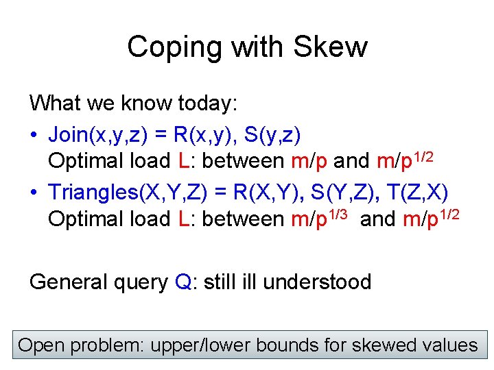
Coping with Skew What we know today: • Join(x, y, z) = R(x, y), S(y, z) Optimal load L: between m/p and m/p 1/2 • Triangles(X, Y, Z) = R(X, Y), S(Y, Z), T(Z, X) Optimal load L: between m/p 1/3 and m/p 1/2 General query Q: still understood Open problem: upper/lower bounds for skewed values 48

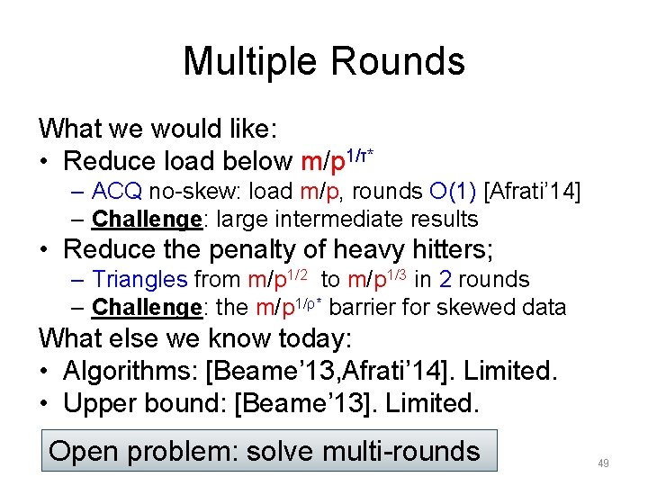
Multiple Rounds What we would like: • Reduce load below m/p 1/τ* – ACQ no-skew: load m/p, rounds O(1) [Afrati’ 14] – Challenge: large intermediate results • Reduce the penalty of heavy hitters; – Triangles from m/p 1/2 to m/p 1/3 in 2 rounds – Challenge: the m/p 1/ρ* barrier for skewed data What else we know today: • Algorithms: [Beame’ 13, Afrati’ 14]. Limited. • Upper bound: [Beame’ 13]. Limited. Open problem: solve multi-rounds 49

More Resources • Extended slides, exercises, open problems: Ph. D Open Warsaw, March 2015 phdopen. mimuw. edu. pl/index. php? page=l 15 w 1 or search for ‘phd open dan suciu’ • Papers: Beame, Koutris, S, [PODS’ 13, 14] Chu, Balazinska, S. [SIGMOD’ 15] • Myria website: myria. cs. washington. edu/ Thank you! 50