Common Signals in MATLAB Prof Brian L Evans

Common Signals in MATLAB Prof. Brian L. Evans Dept. of Electrical and Computer Engineering The University of Texas at Austin Spring 2019

Outline • MATLAB • Mathematical Representations of Signals • Continuous-Time Signals Sinusoids Exponentials Infinite and finite length Sinc pulse Chirps • Spectrograms • Discrete-Time Signals 1 -2

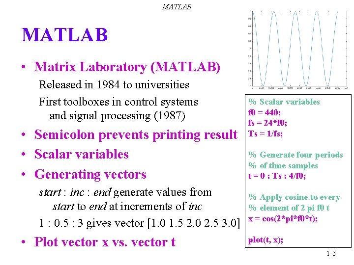
MATLAB • Matrix Laboratory (MATLAB) Released in 1984 to universities First toolboxes in control systems and signal processing (1987) • Semicolon prevents printing result • Scalar variables • Generating vectors start : inc : end generate values from start to end at increments of inc 1 : 0. 5 : 3 gives vector [1. 0 1. 5 2. 0 2. 5 3. 0] • Plot vector x vs. vector t % Scalar variables f 0 = 440; fs = 24*f 0; Ts = 1/fs; % Generate four periods % of time samples t = 0 : Ts : 4/f 0; % Apply cosine to every % element of 2 pi f 0 t x = cos(2*pi*f 0*t); plot(t, x); 1 -3

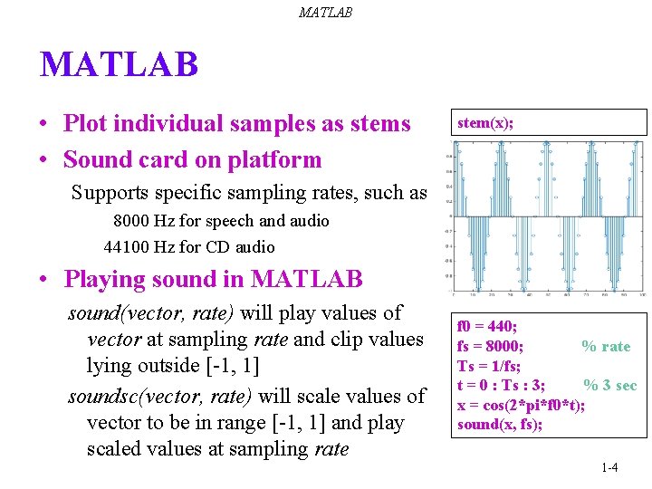
MATLAB • Plot individual samples as stems • Sound card on platform stem(x); Supports specific sampling rates, such as 8000 Hz for speech and audio 44100 Hz for CD audio • Playing sound in MATLAB sound(vector, rate) will play values of vector at sampling rate and clip values lying outside [-1, 1] soundsc(vector, rate) will scale values of vector to be in range [-1, 1] and play scaled values at sampling rate f 0 = 440; fs = 8000; % rate Ts = 1/fs; t = 0 : Ts : 3; % 3 sec x = cos(2*pi*f 0*t); sound(x, fs); 1 -4

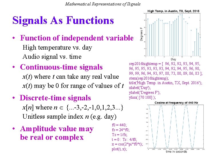
Mathematical Representations of Signals As Functions • Function of independent variable High temperature vs. day Audio signal vs. time • Continuous-time signals x(t) where t can take any real value x(t) may be 0 for range of values of t • Discrete-time signals sep 2016 hightemp = [ 96, 92, 93, 94, 95, 96, 95, 93, 93, 94, 92, 94, 95, 96, 98, 99, 96, 94, 93, 97, 88, 73, 80, 89, 86, 83 ]; stem(sep 2016 hightemp); title('High Temp. in Austin, TX, Sept. 2016'); xlabel('Day'); ylabel('Degrees F'); ylim( [70 100] ); x[n] where n {. . . -3, -2, -1, 0, 1, 2, 3. . . } Unitless sample index n (e. g. day) • Amplitude value may be real or complex f 0 = 440; fs = 24*f 0; Ts = 1/fs; t = 0 : Ts : 4/f 0; x = cos(2*pi*f 0*t); plot(t, x);

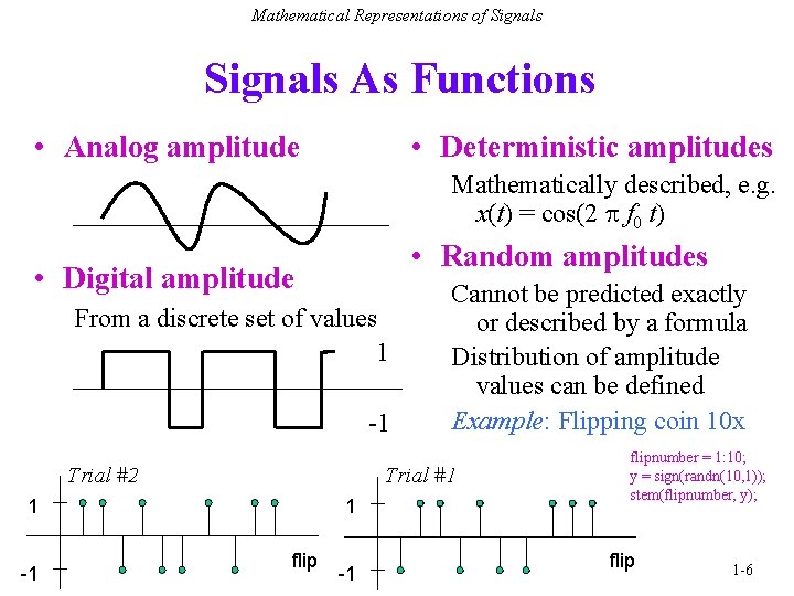
Mathematical Representations of Signals As Functions • Analog amplitude • Deterministic amplitudes Mathematically described, e. g. x(t) = cos(2 f 0 t) • Random amplitudes • Digital amplitude From a discrete set of values 1 -1 Trial #2 1 -1 Cannot be predicted exactly or described by a formula Distribution of amplitude values can be defined Example: Flipping coin 10 x 1 flip -1 flipnumber = 1: 10; y = sign(randn(10, 1)); stem(flipnumber, y); flip 1 -6

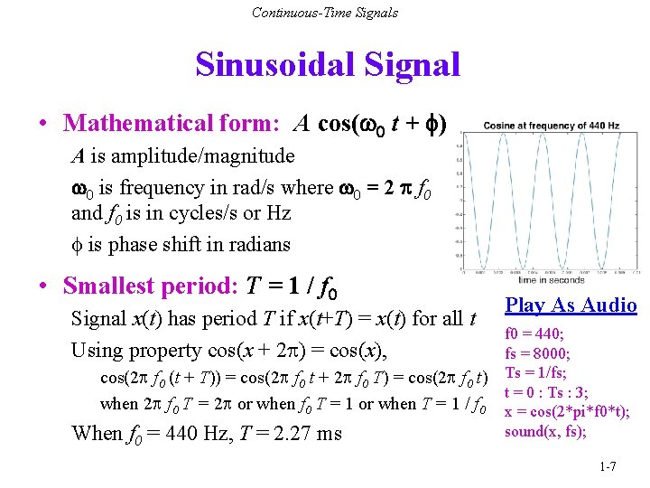
Continuous-Time Signals Sinusoidal Signal • Mathematical form: A cos(w 0 t + f) A is amplitude/magnitude w 0 is frequency in rad/s where w 0 = 2 p f 0 and f 0 is in cycles/s or Hz f is phase shift in radians • Smallest period: T = 1 / f 0 Signal x(t) has period T if x(t+T) = x(t) for all t Using property cos(x + 2 ) = cos(x), cos(2 f 0 (t + T)) = cos(2 f 0 t + 2 f 0 T) = cos(2 f 0 t) when 2 f 0 T = 2 or when f 0 T = 1 or when T = 1 / f 0 When f 0 = 440 Hz, T = 2. 27 ms Play As Audio f 0 = 440; fs = 8000; Ts = 1/fs; t = 0 : Ts : 3; x = cos(2*pi*f 0*t); sound(x, fs); 1 -7

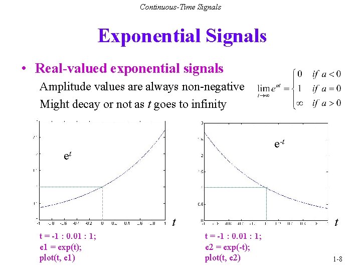
Continuous-Time Signals Exponential Signals • Real-valued exponential signals Amplitude values are always non-negative Might decay or not as t goes to infinity e-t et t t = -1 : 0. 01 : 1; e 1 = exp(t); plot(t, e 1) t t = -1 : 0. 01 : 1; e 2 = exp(-t); plot(t, e 2) 1 -8

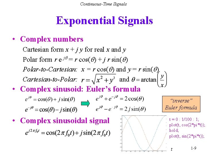
Continuous-Time Signals Exponential Signals • Complex numbers Cartesian form x + j y for real x and y Polar form r e jq = r cos(q) + j r sin(q) Polar-to-Cartesian: x = r cos(q) and y = r sin(q) Cartesian-to-Polar: and • Complex sinusoid: Euler’s formula “inverse” Euler formula • Complex sinusoidal signal t = 0 : 1/100 : 1; plot(t, cos(2*pi*t)); hold; plot(t, sin(2*pi*t)); t 1 -9

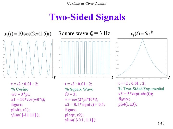
Continuous-Time Signals Two-Sided Signals Square wave f 0 = 3 Hz t t = -2 : 0. 01 : 2; % Cosine w 0 = 3*pi; x 1 = 10*cos(w 0*t); figure; plot(t, x 1); ylim( [-11 11] ); t t t = -2 : 0. 01 : 2; % Square Wave f 0 = 3; v = cos(2*pi*f 0*t); x 2 = 0. 5*sign(v) + 0. 5; figure; plot(t, x 2); ylim( [-0. 1, 1. 1] ); t = -2 : 0. 01 : 2; % Two-Sided Exponential x 3 = 5*exp(-abs(t)); figure; plot(t, x 3); 1 -10

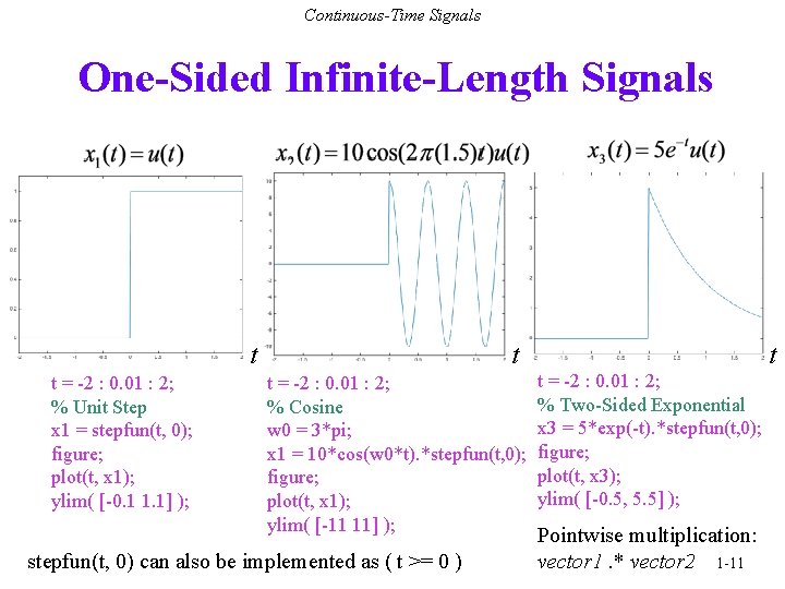
Continuous-Time Signals One-Sided Infinite-Length Signals t t = -2 : 0. 01 : 2; % Unit Step x 1 = stepfun(t, 0); figure; plot(t, x 1); ylim( [-0. 1 1. 1] ); t t = -2 : 0. 01 : 2; % Cosine w 0 = 3*pi; x 1 = 10*cos(w 0*t). *stepfun(t, 0); figure; plot(t, x 1); ylim( [-11 11] ); stepfun(t, 0) can also be implemented as ( t >= 0 ) t t = -2 : 0. 01 : 2; % Two-Sided Exponential x 3 = 5*exp(-t). *stepfun(t, 0); figure; plot(t, x 3); ylim( [-0. 5, 5. 5] ); Pointwise multiplication: vector 1. * vector 2 1 -11

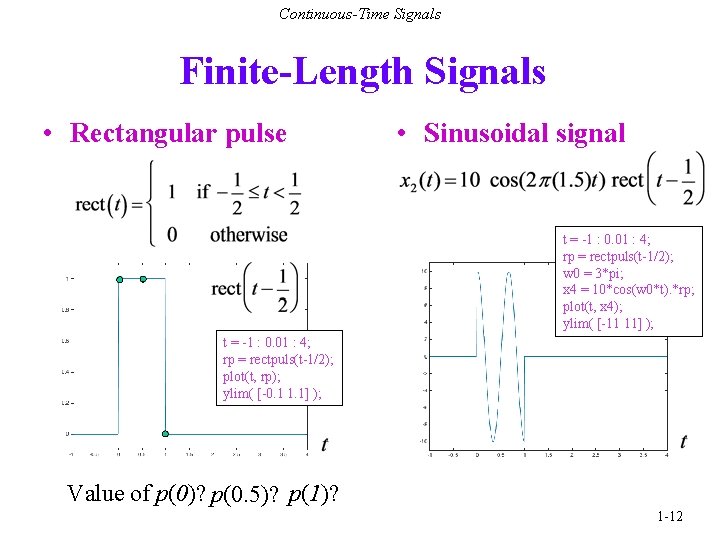
Continuous-Time Signals Finite-Length Signals • Rectangular pulse • Sinusoidal signal t = -1 : 0. 01 : 4; rp = rectpuls(t-1/2); w 0 = 3*pi; x 4 = 10*cos(w 0*t). *rp; plot(t, x 4); ylim( [-11 11] ); t = -1 : 0. 01 : 4; rp = rectpuls(t-1/2); plot(t, rp); ylim( [-0. 1 1. 1] ); Value of p(0)? p(0. 5)? p(1)? 1 -12

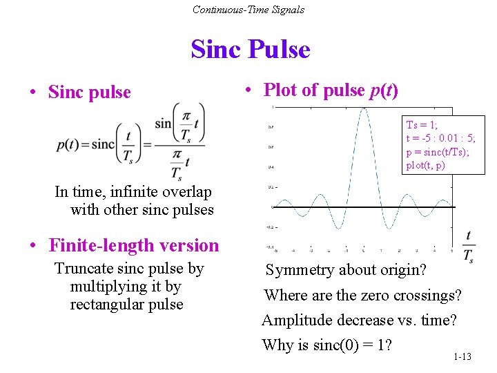
Continuous-Time Signals Sinc Pulse • Sinc pulse • Plot of pulse p(t) Ts = 1; t = -5 : 0. 01 : 5; p = sinc(t/Ts); plot(t, p) In time, infinite overlap with other sinc pulses • Finite-length version Truncate sinc pulse by multiplying it by rectangular pulse Symmetry about origin? Where are the zero crossings? Amplitude decrease vs. time? Why is sinc(0) = 1? 1 -13

Continuous-Time Signals Chirp Signals • Sinusoid with rising or falling frequency vs. time Change in frequency occurs continuously Linear sweep over range of frequencies (e. g. audio test signal) • Revisit sinusoidal signal model Assumes constant amplitude, frequency and phase over time Angle in right term y(t) = 2 f 0 t + f varies linearly with time Derivative of y(t) w/r to t is constant frequency 2 f 0 in rad/s 1 -14

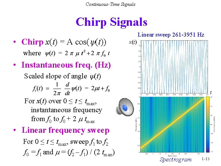
Continuous-Time Signals Chirp Signals • Chirp x(t) = A cos(y(t)) Linear sweep 261 -3951 Hz x(t) where • Instantaneous freq. (Hz) Scaled slope of angle y(t) t For x(t) over 0 ≤ tmax, instantaneous frequency from f 0 to f 0 + 2 m tmax • Linear frequency sweep For 0 ≤ tmax, sweep f 1 to f 2 f 0 = f 1 and m = (f 2 – f 1) / (2 tmax) Spectrogram 1 -15

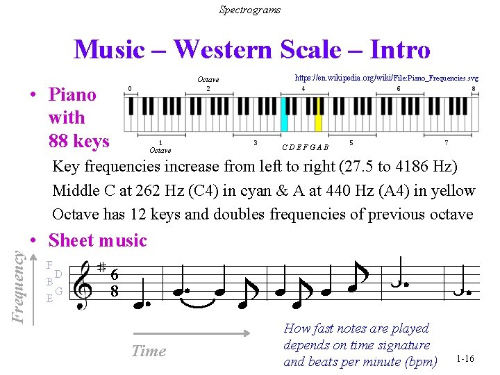
Spectrograms Music – Western Scale – Intro Octave • Piano with 88 keys Octave https: //en. wikipedia. org/wiki/ File: Piano_Frequencies. svg CDEFGAB Frequency Key frequencies increase from left to right (27. 5 to 4186 Hz) Middle C at 262 Hz (C 4) in cyan & A at 440 Hz (A 4) in yellow Octave has 12 keys and doubles frequencies of previous octave • Sheet music F D B G E ♯ 6 8 ♩ ♪ ♩ ♩ ♩ ♪ ♪ ♩ Time How fast notes are played depends on time signature and beats per minute (bpm) 1 -16

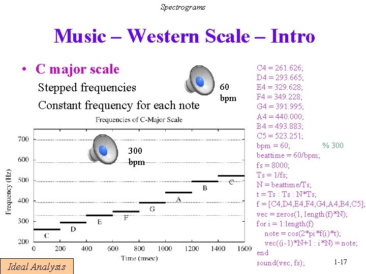
Spectrograms Music – Western Scale – Intro • C major scale Stepped frequencies Constant frequency for each note 300 bpm Ideal Analysis 60 bpm C 4 = 261. 626; D 4 = 293. 665; E 4 = 329. 628; F 4 = 349. 228; G 4 = 391. 995; A 4 = 440. 000; B 4 = 493. 883; C 5 = 523. 251; bpm = 60; % 300 beattime = 60/bpm; fs = 8000; Ts = 1/fs; N = beattime/Ts; t = Ts : N*Ts; f = [C 4, D 4, E 4, F 4, G 4, A 4, B 4, C 5]; vec = zeros(1, length(f)*N); for i = 1: length(f) note = cos(2*pi*f(i)*t); vec((i-1)*N+1 : i*N) = note; end 1 -17 sound(vec, fs);

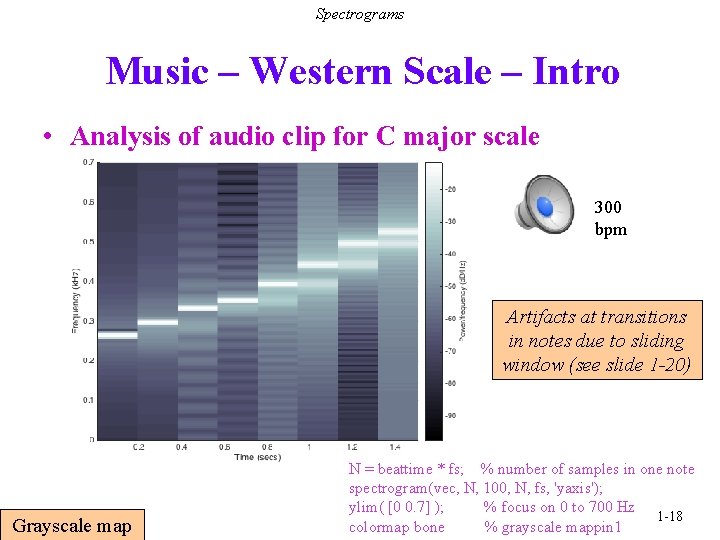
Spectrograms Music – Western Scale – Intro • Analysis of audio clip for C major scale 300 bpm Artifacts at transitions in notes due to sliding window (see slide 1 -20) Grayscale map N = beattime * fs; % number of samples in one note spectrogram(vec, N, 100, N, fs, 'yaxis'); ylim( [0 0. 7] ); % focus on 0 to 700 Hz 1 -18 colormap bone % grayscale mappin 1

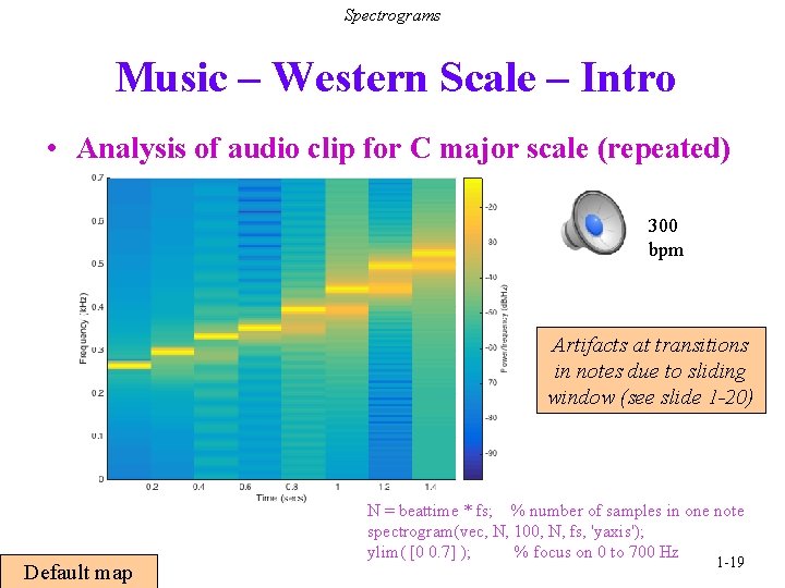
Spectrograms Music – Western Scale – Intro • Analysis of audio clip for C major scale (repeated) 300 bpm Artifacts at transitions in notes due to sliding window (see slide 1 -20) Default map N = beattime * fs; % number of samples in one note spectrogram(vec, N, 100, N, fs, 'yaxis'); ylim( [0 0. 7] ); % focus on 0 to 700 Hz 1 -19

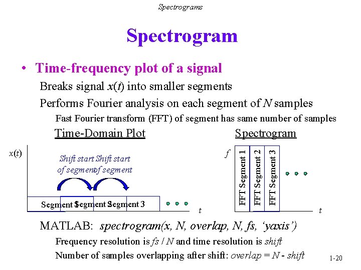
Spectrograms Spectrogram • Time-frequency plot of a signal Breaks signal x(t) into smaller segments Performs Fourier analysis on each segment of N samples Fast Fourier transform (FFT) of segment has same number of samples Segment S 1 egment S 2 egment 3 t FFT Segment 3 f Shift start of segment FFT Segment 2 x(t) FFT Segment 1 Spectrogram Time-Domain Plot t MATLAB: spectrogram(x, N, overlap, N, fs, ‘yaxis’) Frequency resolution is fs / N and time resolution is shift Number of samples overlapping after shift: overlap = N - shift 1 -20

Discrete-Time Signals & Systems • Discrete-time signals (see slide 2 -9) Formula: x[n] = cos(( /2) n) useful in analysis Samples: xvec = [1 0 -1 0] useful in simulation Properties: even symmetric useful in reasoning Piecewise: v[n] = rectpuls(n/10) • Discrete-time systems Produce output signal from input signal x[n] T{ • } y[n] Squaring: y[n] = x 2[n] Averaging: y[n] = ½ x[n] + ½ x[n-1] n = -7 : 7; v = rectpuls(n/10); stem(n, v); Width is 10 samples 1 -21

Discrete-Time Signals Unit Impulse Response • Discrete-time unit impulse signal d[n] d[n-2] 1 -3 -2 -1 1 0 1 2 3 n -3 -2 -1 0 1 2 3 n • Expressing finite-length signals using unit impulses 3 d[n] 2 d[n+1] 2 d[n-1] 2 d[n+2] -3 x[n] 3 d[n-2] 1 -2 -1 0 1 2 No MATLAB function for d[n] Could use rectpuls(n) but awkward 3 n n = -3 : 3; x = [0 1 2 3 2 1 0]; stem(n, x); - OR n = -3 : 3; x = 3*tripuls(n/6); stem(n, x); 1 -22

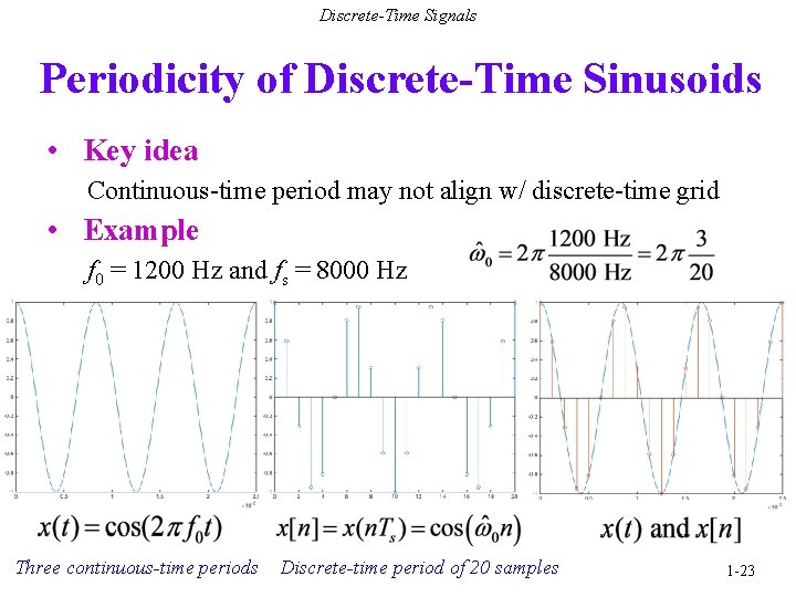
Discrete-Time Signals Periodicity of Discrete-Time Sinusoids • Key idea Continuous-time period may not align w/ discrete-time grid • Example f 0 = 1200 Hz and fs = 8000 Hz Three continuous-time periods Discrete-time period of 20 samples 1 -23

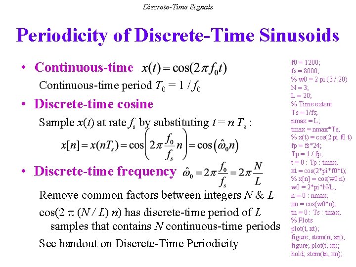
Discrete-Time Signals Periodicity of Discrete-Time Sinusoids • Continuous-time period T 0 = 1 / f 0 • Discrete-time cosine Sample x(t) at rate fs by substituting t = n Ts : • Discrete-time frequency Remove common factors between integers N & L cos(2 (N / L) n) has discrete-time period of L samples that contains N continuous-time periods See handout on Discrete-Time Periodicity f 0 = 1200; fs = 8000; % w 0 = 2 pi (3 / 20) N = 3; L = 20; % Time extent Ts = 1/fs; nmax = L; tmax = nmax*Ts; % x(t) = cos(2 pi f 0 t) fp = fs*24; Tp = 1 / fp; t = 0 : Tp : tmax; xt = cos(2*pi*f 0*t); % x[n] = cos(w 0 n) w 0 = 2*pi*N/L; n = 0 : nmax; xn = cos(w 0*n); tn = 0 : Ts : tmax; % Plots plot(t, xt); figure; stem(n, xn); figure; plot(t, xt); hold; stem(tn, xn);