Common Families of Probability Distributions Bernoulli Distribution An

Common Families of Probability Distributions

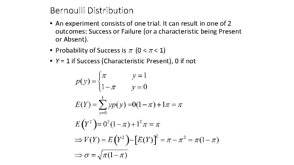
Bernoulli Distribution • An experiment consists of one trial. It can result in one of 2 outcomes: Success or Failure (or a characteristic being Present or Absent). • Probability of Success is p (0 < p < 1) • Y = 1 if Success (Characteristic Present), 0 if not

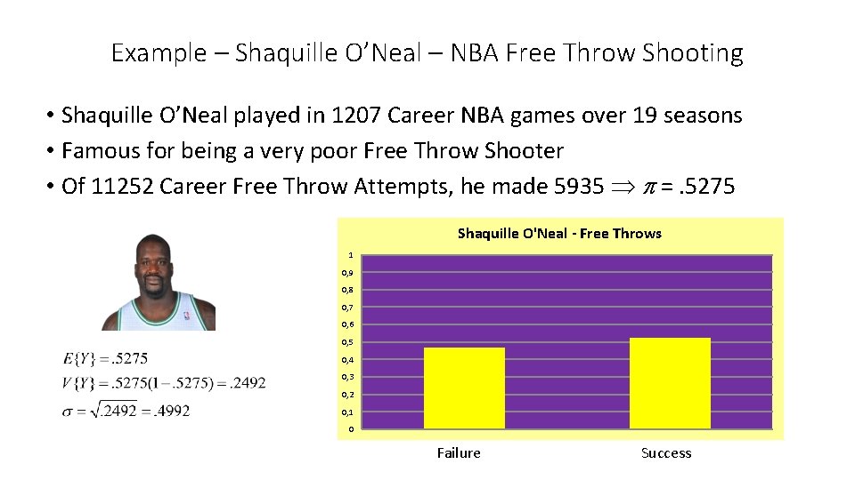
Example – Shaquille O’Neal – NBA Free Throw Shooting • Shaquille O’Neal played in 1207 Career NBA games over 19 seasons • Famous for being a very poor Free Throw Shooter • Of 11252 Career Free Throw Attempts, he made 5935 p =. 5275 Shaquille O'Neal - Free Throws 1 0, 9 0, 8 0, 7 0, 6 0, 5 0, 4 0, 3 0, 2 0, 1 0 Failure Success

Binomial Distribution

Binomial Experiment • Experiment consists of a series of n identical trials • Each trial can end in one of 2 outcomes: Success or Failure • Trials are independent (outcome of one has no bearing on outcomes of others) • Probability of Success, p, is constant for all trials • Random Variable Y, is the number of Successes in the n trials is said to follow Binomial Distribution with parameters n and p • Y can take on the values y=0, 1, …, n Notation: Y~Bin(n, p) EXCEL: =BINOM. DIST(y, n, p, 1) gives P(Y<=y) =BINOM. DIST(y, n, p, 0) gives p(y)=P(Y=y)

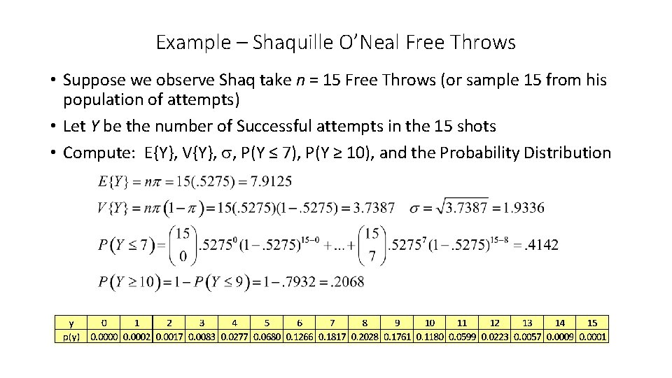
Example – Shaquille O’Neal Free Throws • Suppose we observe Shaq take n = 15 Free Throws (or sample 15 from his population of attempts) • Let Y be the number of Successful attempts in the 15 shots • Compute: E{Y}, V{Y}, s, P(Y ≤ 7), P(Y ≥ 10), and the Probability Distribution

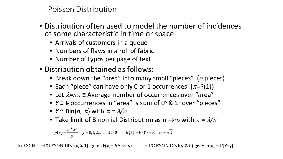
Poisson Distribution • Distribution often used to model the number of incidences of some characteristic in time or space: • Arrivals of customers in a queue • Numbers of flaws in a roll of fabric • Number of typos per page of text. • Distribution obtained as follows: • • • Break down the “area” into many small “pieces” (n pieces) Each “piece” can have only 0 or 1 occurrences (p=P(1)) Let l=np ≡ Average number of occurrences over “area” Y ≡ # occurrences in “area” is sum of 0 s & 1 s over “pieces” Y ~ Bin(n, p) with p = l/n Take limit of Binomial Distribution as n with p = l/n In EXCEL: =POISSON. DIST(y, l, 1) gives F(y)=P(Y <= y) = POISSON. DIST(y, l, 0) gives p(y) = P(Y=y)

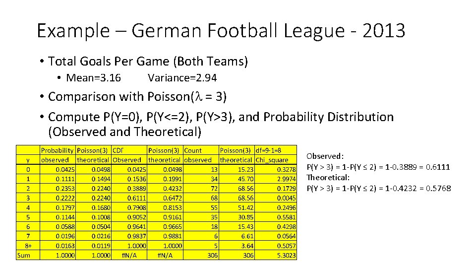
Example – German Football League - 2013 • Total Goals Per Game (Both Teams) • Mean=3. 16 Variance=2. 94 • Comparison with Poisson(l = 3) • Compute P(Y=0), P(Y<=2), P(Y>3), and Probability Distribution (Observed and Theoretical) Observed: P(Y > 3) = 1 -P(Y ≤ 2) = 1 -0. 3889 = 0. 6111 Theoretical: P(Y > 3) = 1 -P(Y ≤ 2) = 1 -0. 4232 = 0. 5768

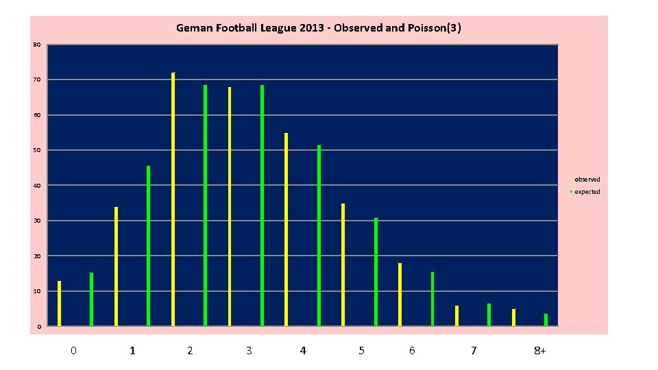
Geman Football League 2013 - Observed and Poisson(3) 80 70 60 50 observed 40 expected 30 20 10 0 0 1 2 3 4 5 6 7 8+

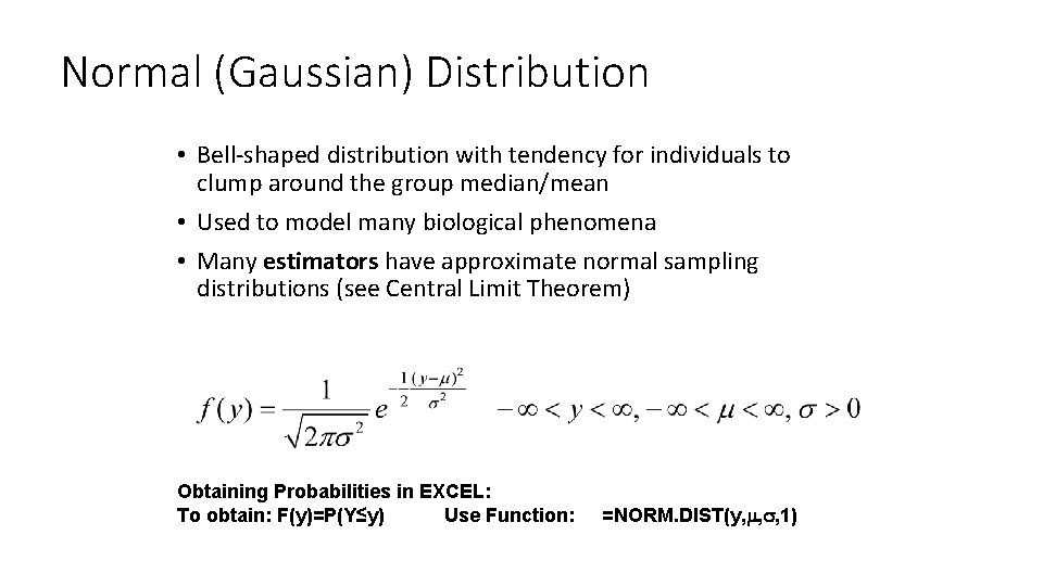
Normal (Gaussian) Distribution • Bell-shaped distribution with tendency for individuals to clump around the group median/mean • Used to model many biological phenomena • Many estimators have approximate normal sampling distributions (see Central Limit Theorem) Obtaining Probabilities in EXCEL: To obtain: F(y)=P(Y≤y) Use Function: =NORM. DIST(y, m, s, 1)

Normal Distribution – Density Functions (pdf)

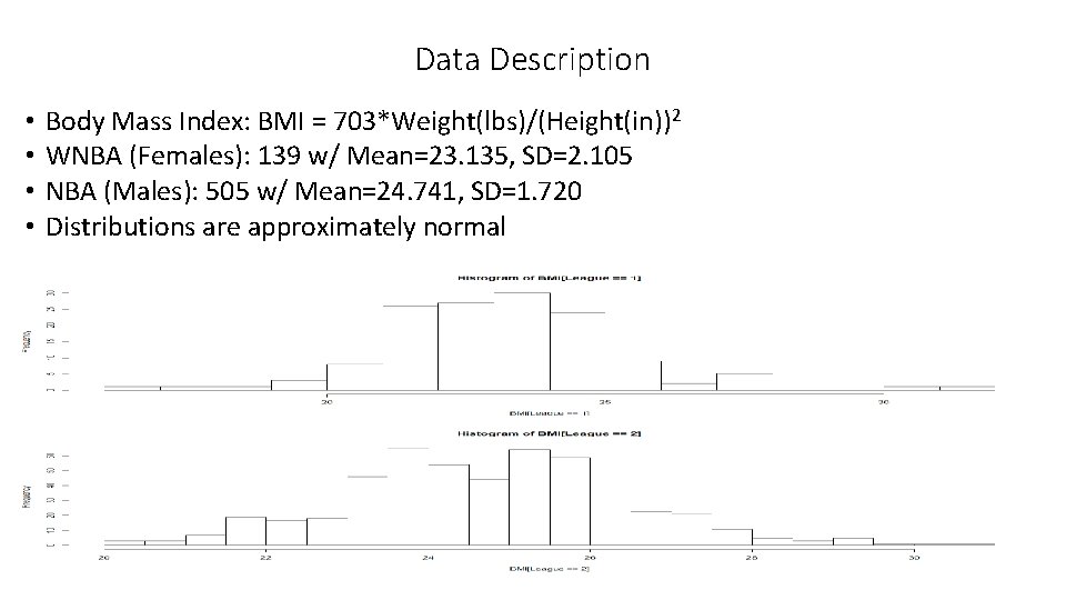
Data Description • • Body Mass Index: BMI = 703*Weight(lbs)/(Height(in))2 WNBA (Females): 139 w/ Mean=23. 135, SD=2. 105 NBA (Males): 505 w/ Mean=24. 741, SD=1. 720 Distributions are approximately normal

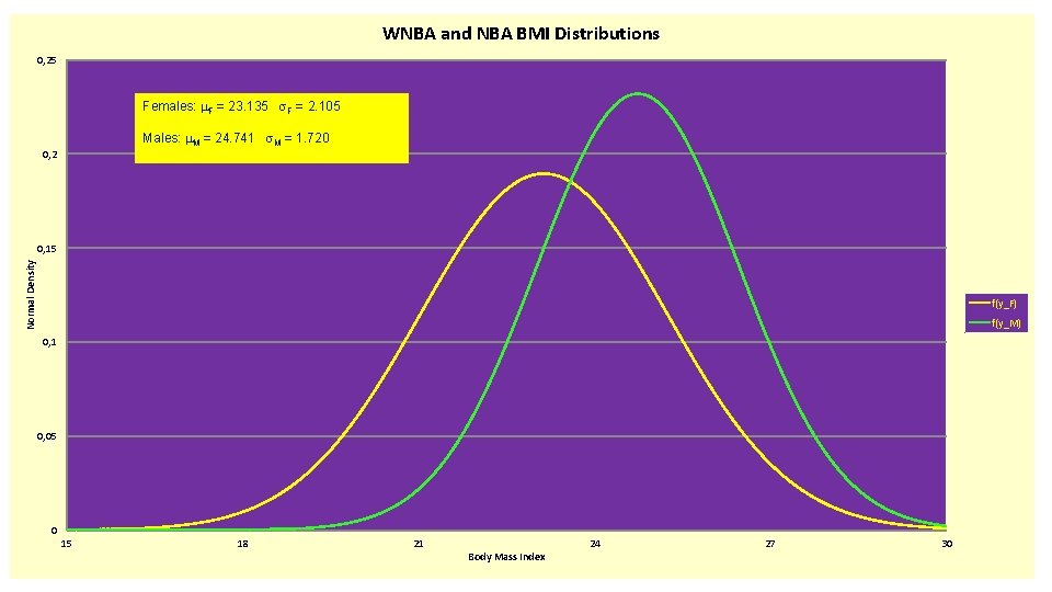
WNBA and NBA BMI Distributions 0, 25 Females: m. F = 23. 135 s. F = 2. 105 Males: m. M = 24. 741 s. M = 1. 720 0, 2 Normal Density 0, 15 f(y_F) f(y_M) 0, 1 0, 05 0 15 18 21 Body Mass Index 24 27 30

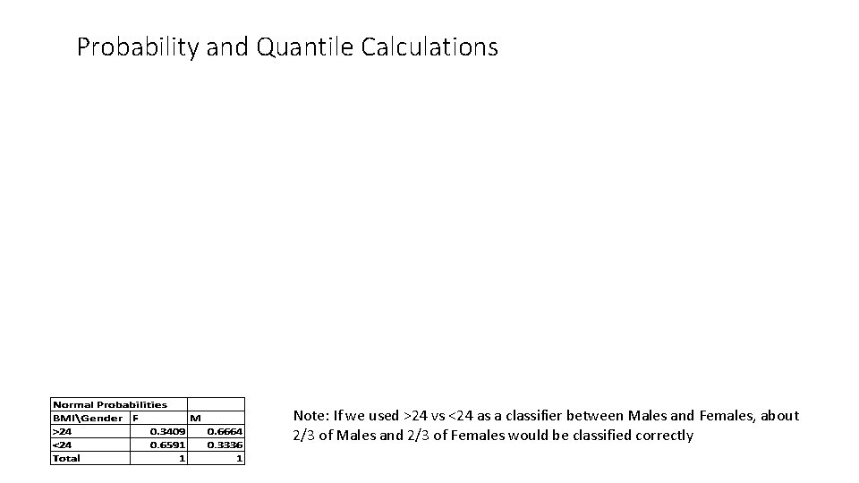
Probability and Quantile Calculations Note: If we used >24 vs <24 as a classifier between Males and Females, about 2/3 of Males and 2/3 of Females would be classified correctly

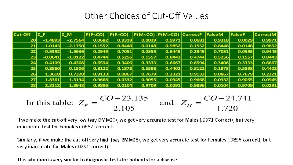
Other Choices of Cut-Off Values If we make the cut-off very low (say BMI=20), we get very accurate test for Males (. 9971 Correct), but very inaccurate test for Females (. 0682) correct. Similarly, if we make the cut-off very high (say BMI=28), we get very accurate test for Females (. 9896 correct), but very inaccurate for Males (. 0291 correct) This situation is very similar to diagnostic tests for patients for a disease

Prior/Posterior Probabilities, Odds, Likelihood Ratios

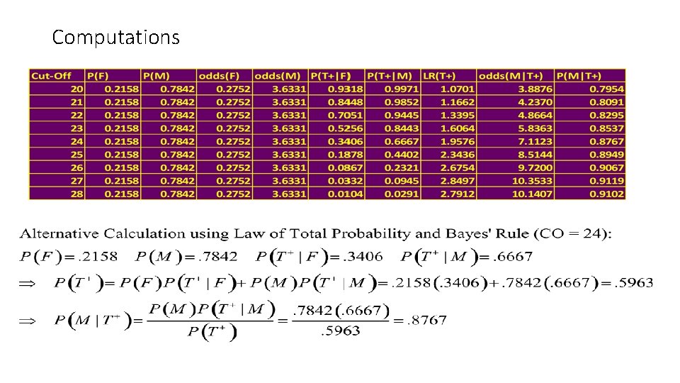
Computations

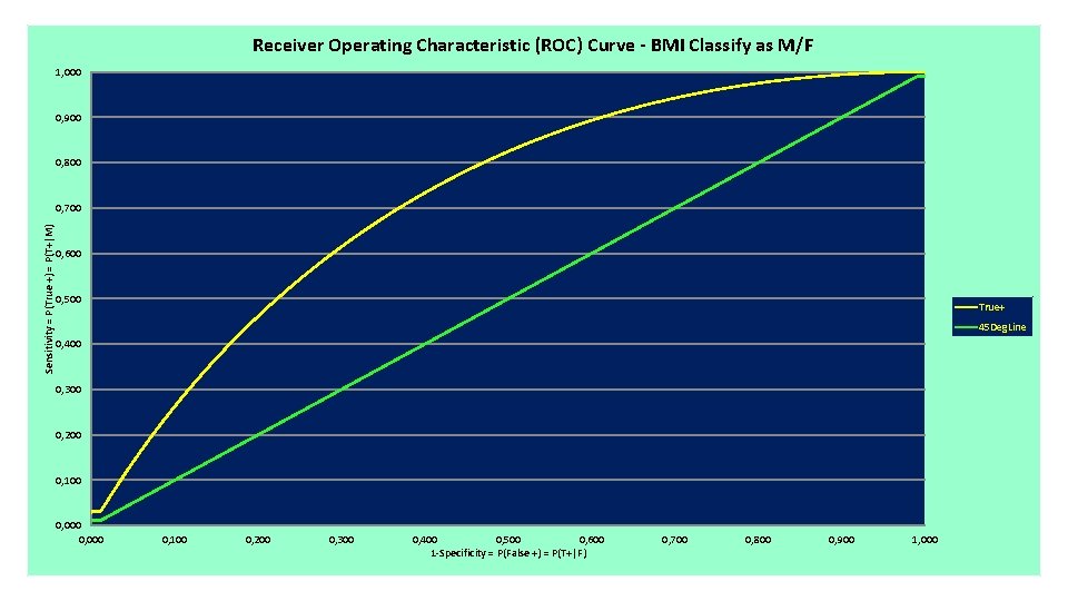
Receiver Operating Characteristic (ROC) Curve - BMI Classify as M/F 1, 000 0, 900 0, 800 Sensitivity = P(True +) = P(T+|M) 0, 700 0, 600 0, 500 True+ 45 Deg. Line 0, 400 0, 300 0, 200 0, 100 0, 000 0, 100 0, 200 0, 300 0, 400 0, 500 0, 600 1 -Specificity = P(False +) = P(T+|F) 0, 700 0, 800 0, 900 1, 000

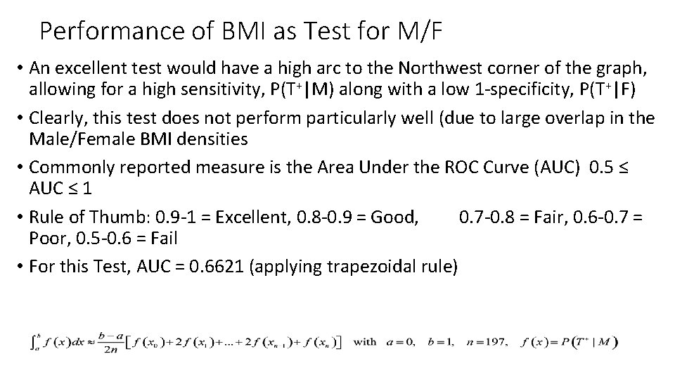
Performance of BMI as Test for M/F • An excellent test would have a high arc to the Northwest corner of the graph, allowing for a high sensitivity, P(T+|M) along with a low 1 -specificity, P(T+|F) • Clearly, this test does not perform particularly well (due to large overlap in the Male/Female BMI densities • Commonly reported measure is the Area Under the ROC Curve (AUC) 0. 5 ≤ AUC ≤ 1 • Rule of Thumb: 0. 9 -1 = Excellent, 0. 8 -0. 9 = Good, 0. 7 -0. 8 = Fair, 0. 6 -0. 7 = Poor, 0. 5 -0. 6 = Fail • For this Test, AUC = 0. 6621 (applying trapezoidal rule)

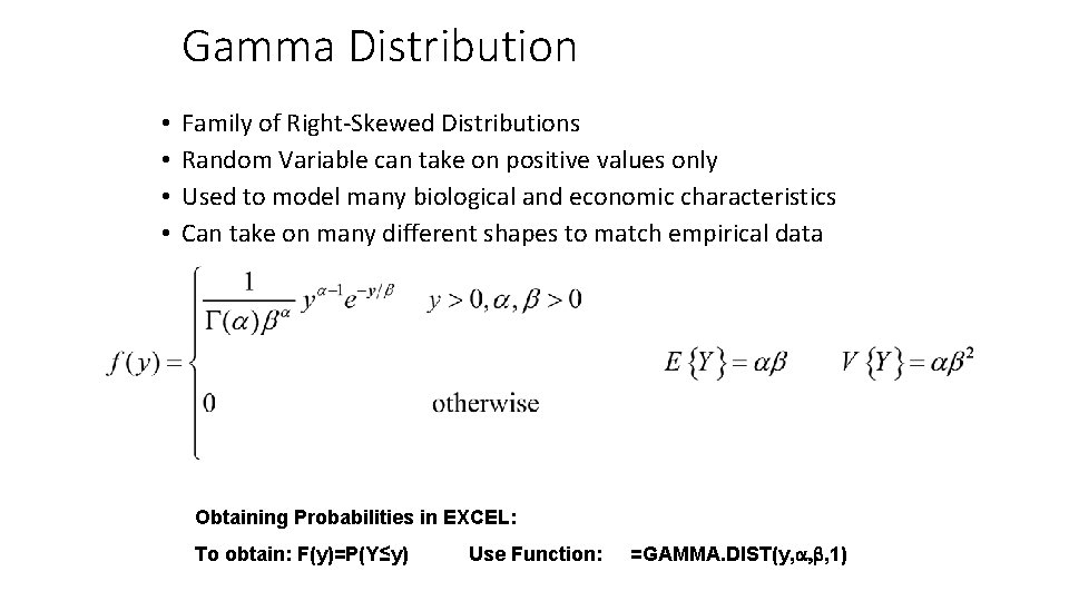
Gamma Distribution • • Family of Right-Skewed Distributions Random Variable can take on positive values only Used to model many biological and economic characteristics Can take on many different shapes to match empirical data Obtaining Probabilities in EXCEL: To obtain: F(y)=P(Y≤y) Use Function: =GAMMA. DIST(y, a, b, 1)

Gamma/Exponential Densities (pdf)

Lognormal Distribution Obtaining Probabilities in EXCEL: To obtain: F(y)=P(Y≤y) Use Function: =LOGNORM. DIST(y, m, s, 1))

Lognormal pdf’s

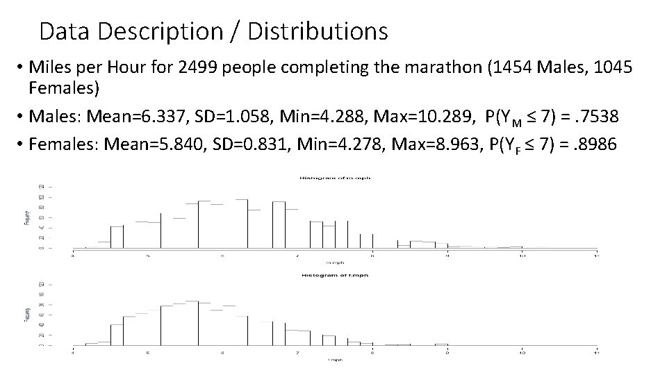
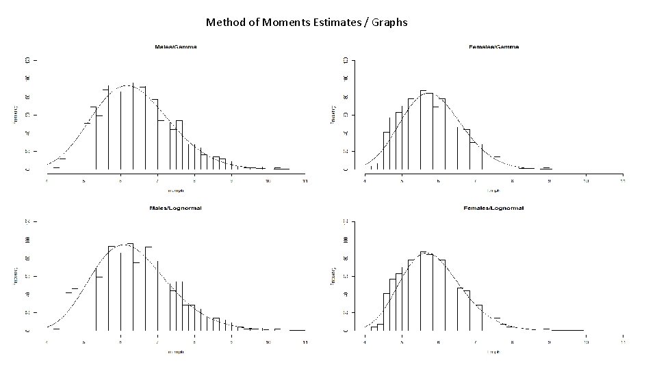
Data Description / Distributions • Miles per Hour for 2499 people completing the marathon (1454 Males, 1045 Females) • Males: Mean=6. 337, SD=1. 058, Min=4. 288, Max=10. 289, P(YM ≤ 7) =. 7538 • Females: Mean=5. 840, SD=0. 831, Min=4. 278, Max=8. 963, P(YF ≤ 7) =. 8986

Method of Moments Estimators - Gamma Obtain the Sample Mean and Variance and Use them to obtain estimates of parameters and P(Y ≤ 7)

Method of Moments Estimators - Lognormal

Method of Moments Estimates / Graphs