Common conservation and management models Biomassdynamics models logistic

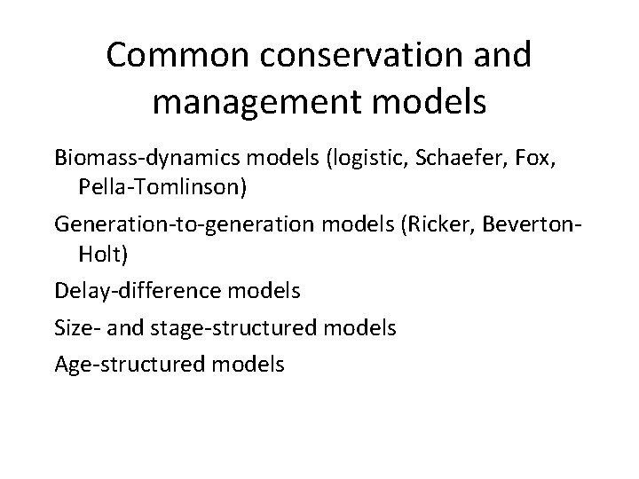
Common conservation and management models Biomass-dynamics models (logistic, Schaefer, Fox, Pella-Tomlinson) Generation-to-generation models (Ricker, Beverton. Holt) Delay-difference models Size- and stage-structured models Age-structured models

Models with no age structure • • Exponential growth Logistic model (or “Schaefer” model) Fox model Pella-Tomlinson model Schaefer MB (1954) Some aspects of the dynamics of the population important to the management of the commercial marine fisheries. Inter. American Tropical Tuna Commission Bulletin 1: 25 -56 Fox WW (1970) An exponential surplus-yield model for optimizing exploited fish populations. Trans. American Fisheries Society 99: 80 -88 Pella JJ & Tomlinson PK (1969) A generalized stock production model. Inter-American Tropical Tuna Commission Bulletin 13: 419 -496

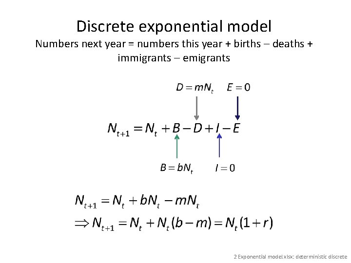
Discrete exponential model Numbers next year = numbers this year + births – deaths + immigrants – emigrants 2 Exponential model. xlsx: deterministic discrete

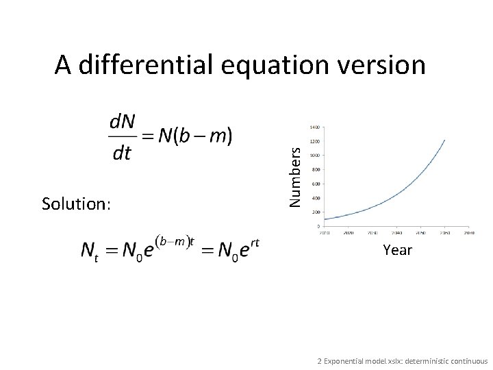
Solution: Numbers A differential equation version Year 2 Exponential model. xslx: deterministic continuous

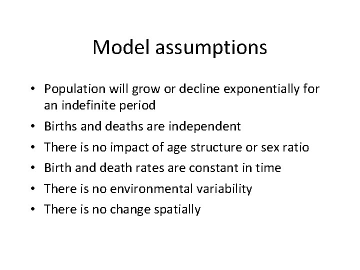
Model assumptions • Population will grow or decline exponentially for an indefinite period • Births and deaths are independent • There is no impact of age structure or sex ratio • Birth and death rates are constant in time • There is no environmental variability • There is no change spatially

Individual-based exponential model For every year For every individual Pick random numbers X 1~U[0, 1], and X 2~U[0, 1] (uniform between 0 and 1) If X 1 < b then a new birth If X 2 < m then individual dies 2 Exponential indiv based. r

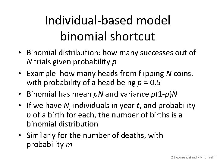
Individual-based model binomial shortcut • Binomial distribution: how many successes out of N trials given probability p • Example: how many heads from flipping N coins, with probability of a head being p = 0. 5 • Binomial has mean p. N and variance p(1 -p)N • If we have Nt individuals in year t, and probability b of a birth for each, the number of births is a binomial distribution • Similarly for the number of deaths, with probability m 2 Exponential indiv binomial. r

2 Exponential indiv based. r

2 Exponential indiv binomial. r

Types of stochasticity Stochasticity means randomness Demographic: random births and deaths Phenotypic: not all individuals are alike Environmental: some years are better than others, El Niño, hurricanes, deep freeze etc. • Spatial: not all places are alike • •

Only demographic stochasticity was included in previous models • We often allow for a more general model of stochasticity: • wt is normally distributed with mean of zero and standard deviation s • numbers next year depend upon numbers this year, the parameters p, any forcing function ut (such as harvesting) and random environmental conditions based on wt

Lognormal error: a little deeper • If wt is normally distributed with mean zero, then exp(wt) is lognormally distributed • When wt = 0, exp(wt) = 1, “average year” • When wt > 0, exp(wt) > 1, “good year” • When wt < 0, exp(wt) < 1, “bad year” • Since exp(wt) is not symmetric, the expected value is not 1 • Therefore we use a correction factor:

Lognormal error correction mean = 0. 003 mean = 1. 646 mean = 1. 0005 You want the mean to be close to 1, since you are multiplying by it 2 Lognormal error hist. r

Continuous exponential model with lognormal error

Number of users (millions) Months since launch https: //www. businessinsider. com. au/chart-of-the-day-google-is-growing-much-faster-than-facebook-did-in-the-early-days-2012 -2

Facebook users (millions) Year Figure by Ben Foster @benphoster

Logistic model Peak catch occurs when B = 0. 5 K Surplus production Biomass at time t+1 Intrinsic (maximum) rate of increase Catch Carrying capacity

“Compensation” • At high densities there will be increasing competition for food, refuges from predators, space, or other critical requirements • Therefore birth rates decline, mortality rates increase, or both • This is called compensation or densitydependence and is measured by the difference between population growth rate when resources are scarce vs. when they are abundant

Surplus production • If surplus production is equal to catch, then the population remains at constant levels • In other words, surplus production is exactly the sustainable catch at a given level of biomass • The highest possible surplus production is called maximum sustainable yield (MSY) • MSY is enshrined in national and international law as a target or limit for fishing

Logistic model Surplus production and maximum sustainable yield (MSY) Surplus production The curve is a symmetrical parabola, which is 0 at B = 0 and B = K, and has a maximum at B = K/2 Biomass (fraction of K) 2 Non-age models. xlsx: Fox vs logistic

Logistic model SP/biomass Rate of population increase is surplus production divided by biomass Biomass (fraction of carrying capacity)

Fox model Peak catch occurs when B = 0. 37 K Surplus production Biomass at time t+1 Intrinsic (maximum) rate of increase Catch Carrying capacity

Logistic vs. Fox model Surplus production Note: Fox model will have lower SP for the same r value Biomass (fraction of K) 2 Non-age models. xlsx: Fox vs logistic

Pella-Tomlinson model Peak catch occurs anywhere from B = 0 to B = K, depending on n Biomass at time t+1 Determines which biomass will yield MSY Catch Surplus production MSY: maximum sustainable yield Carrying capacity

Pella-Tomlinson model These plots all have m = MSY = 500 Surplus production Becomes the Fox model as n 1 Becomes the logistic model when n = 2 Biomass (fraction of K) 2 Non-age models. xlsx: Pella-Tomlinson

Advantages and disadvantages • Logistic, Fox, and Pella-Tomlinson offer different hypotheses about the biomass level at which MSY would be obtained • The Pella-Tomlinson is more flexible but has three parameters instead of two • The most often used is the logistic (know the assumptions and weaknesses) • For fisheries, MSY on average occurs at 0. 4 K, which is a Pella-Tomlinson with n = 2. 39 Thorson et al. (2012) Spawning biomass reference points for exploited marine fishes, incorporating taxonomic and body size information. Canadian Journal of Fisheries and Aquatic Sciences 69: 1556 -1568

Later in the course • Serial autocorrelation: when environmental conditions are not independent in time, but come in runs of good years and runs of bad years more often than would be expected by chance • This results in regime shifts between good periods and bad periods • We will ask whether environment or biomass is a better predictor of surplus production