Committee Machines and Mixtures of Experts Neural Networks

Committee Machines and Mixtures of Experts Neural Networks 12

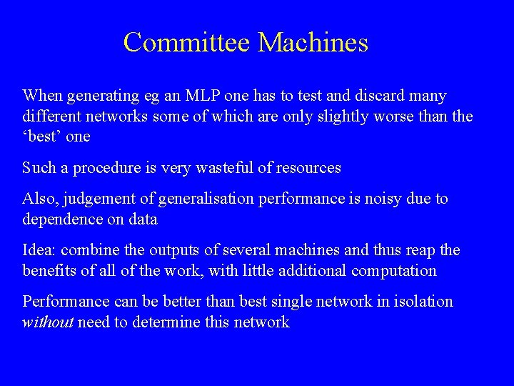
Committee Machines When generating eg an MLP one has to test and discard many different networks some of which are only slightly worse than the ‘best’ one Such a procedure is very wasteful of resources Also, judgement of generalisation performance is noisy due to dependence on data Idea: combine the outputs of several machines and thus reap the benefits of all of the work, with little additional computation Performance can be better than best single network in isolation without need to determine this network

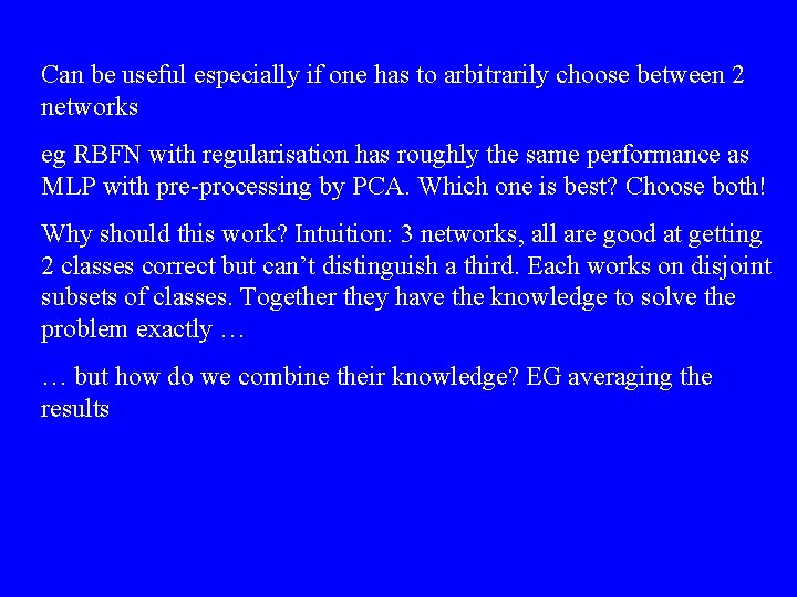
Can be useful especially if one has to arbitrarily choose between 2 networks eg RBFN with regularisation has roughly the same performance as MLP with pre-processing by PCA. Which one is best? Choose both! Why should this work? Intuition: 3 networks, all are good at getting 2 classes correct but can’t distinguish a third. Each works on disjoint subsets of classes. Together they have the knowledge to solve the problem exactly … … but how do we combine their knowledge? EG averaging the results

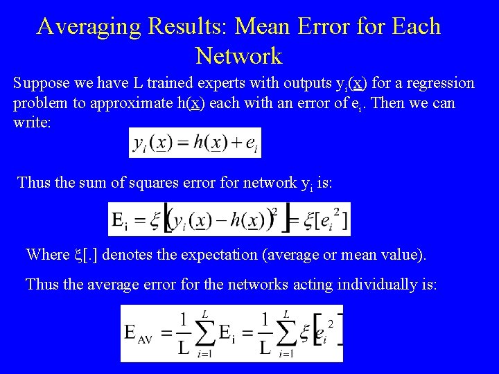
Averaging Results: Mean Error for Each Network Suppose we have L trained experts with outputs yi(x) for a regression problem to approximate h(x) each with an error of ei. Then we can write: Thus the sum of squares error for network yi is: Where x[. ] denotes the expectation (average or mean value). Thus the average error for the networks acting individually is:

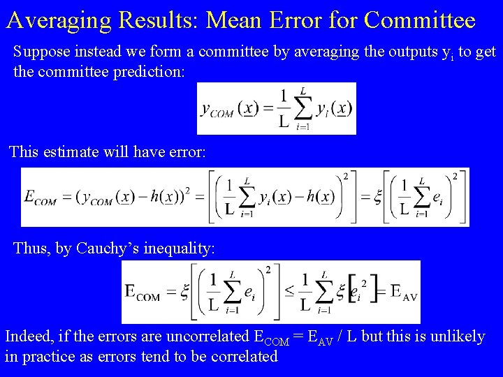
Averaging Results: Mean Error for Committee Suppose instead we form a committee by averaging the outputs yi to get the committee prediction: This estimate will have error: Thus, by Cauchy’s inequality: Indeed, if the errors are uncorrelated ECOM = EAV / L but this is unlikely in practice as errors tend to be correlated

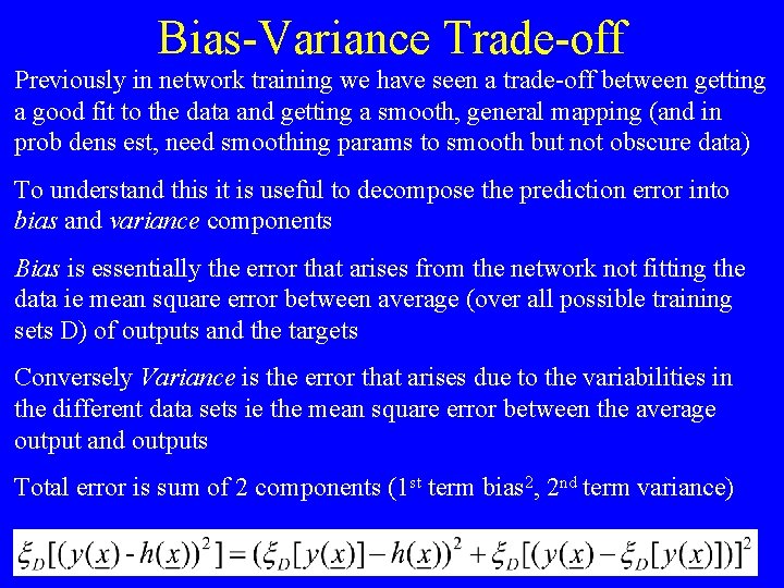
Bias-Variance Trade-off Previously in network training we have seen a trade-off between getting a good fit to the data and getting a smooth, general mapping (and in prob dens est, need smoothing params to smooth but not obscure data) To understand this it is useful to decompose the prediction error into bias and variance components Bias is essentially the error that arises from the network not fitting the data ie mean square error between average (over all possible training sets D) of outputs and the targets Conversely Variance is the error that arises due to the variabilities in the different data sets ie the mean square error between the average output and outputs Total error is sum of 2 components (1 st term bias 2, 2 nd term variance)

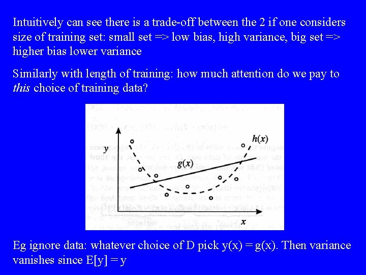
Intuitively can see there is a trade-off between the 2 if one considers size of training set: small set => low bias, high variance, big set => higher bias lower variance Similarly with length of training: how much attention do we pay to this choice of training data? Eg ignore data: whatever choice of D pick y(x) = g(x). Then variance vanishes since E[y] = y

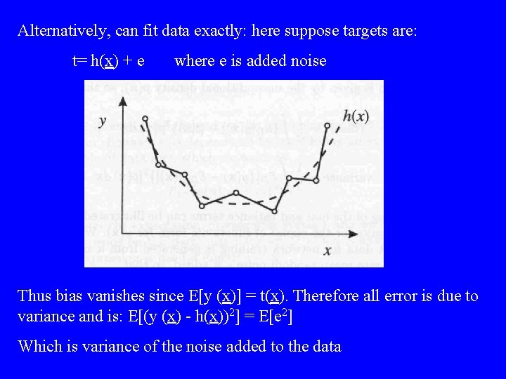
Alternatively, can fit data exactly: here suppose targets are: t= h(x) + e where e is added noise Thus bias vanishes since E[y (x)] = t(x). Therefore all error is due to variance and is: E[(y (x) - h(x))2] = E[e 2] Which is variance of the noise added to the data

The reduction in error can be viewed as coming from a reduction in the variance of each individual network as we are averaging over several networks Þ Each individual net should not have a bias which minimises the bias-variance trade-off but should in fact be overtrained to have a low bias as the extra variance can be removed by averaging Can we do better? What if we weight the average so that members which have better predictions have more input Can be shown, via Lagrange multipliers (pp 367 -369, Bishop) that we can do better and it is best if we increase the spread of predictions of the nets without increasing the errors Intuitively appealing: we want specialised experts (low bias) that specialise on different parts of the problem (spread of predictions)

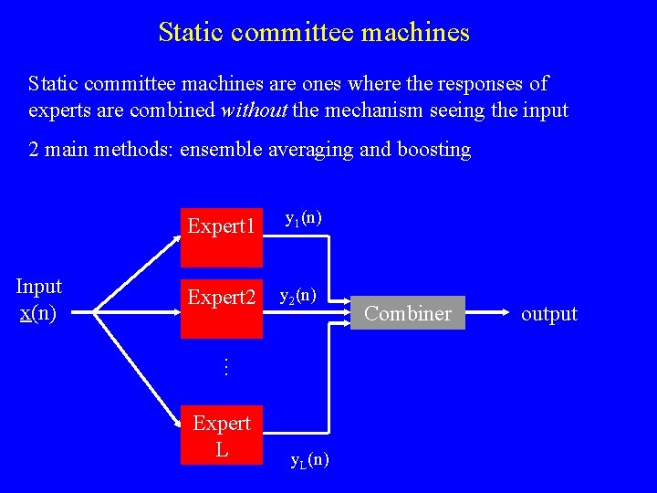
Static committee machines are ones where the responses of experts are combined without the mechanism seeing the input 2 main methods: ensemble averaging and boosting y 1(n) Expert 2 y 2(n) … Input x(n) Expert 1 Expert L y. L(n) Combiner output

Ensemble averaging Perform a weighted average of the outputs (NOT the same as averaging the performance) Why? If weights are all equal, many bad classifiers can outweigh fewer good classifiers Analagous to voting which is used for classification (machnies vote for which class pattern belongs to: most votes wins) However, if weights are based on performance of the machine, one classifier which is wrong but thinks it is right can outweigh many that are right but are not so sure Problematic since we want heterogenous distribution of expertise ie if we have one net which is good apart from on one bit, it will have good performance and so will outweigh another network which knows the bit the first one doesn’t

Boosting In ensemble averaging all nets are trained on the same data In Boosting we generate several different subsets of data and train our possibly weak networks (ie nets whose peformace is slightly more than 50%) on them so that they specialise on different bits Can be used to improve the performance of any learning machine (by eg biasing samples towards difficult examples) Will examine 2 different approaches here: 1. Boosting by filtering. Filter the data via a weak learning machine. Assumes infinite (lots of) data, but low memory requirements 2. Boosting by subsampling. Fixed size data set ‘resampled’ according to some probability distribution during training

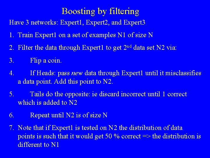
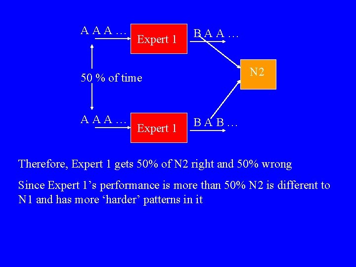
Boosting by filtering Have 3 networks: Expert 1, Expert 2, and Expert 3 1. Train Expert 1 on a set of examples N 1 of size N 2. Filter the data through Expert 1 to get 2 nd data set N 2 via: 3. Flip a coin. 4. If Heads: pass new data through Expert 1 until it misclassifies a data point. Add this point to N 2. 5. Tails do the opposite: ie discard incorrect until 1 correct which is added to N 2 6. Repeat until N 2 is of size N 7. Note that if Expert 1 is tested on N 2 the distribution of data points is such that it would get 50 % correct => the distribution is different to N 1

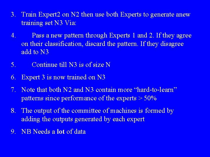
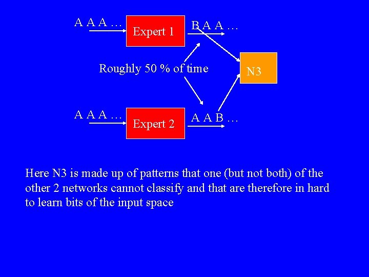
3. Train Expert 2 on N 2 then use both Experts to generate anew training set N 3 Via: 4. 5. Pass a new pattern through Experts 1 and 2. If they agree on their classification, discard the pattern. If they disagree add to N 3 Continue till N 3 is of size N 6. Expert 3 is now trained on N 3 7. Note that both N 2 and N 3 contain more “hard-to-learn” patterns since performance of the experts > 50% 8. The output of the committee of machines is formed by adding the outputs generated by each expert 9. NB Needs a lot of data

AAA… Expert 1 BAA… N 2 50 % of time AAA… Expert 1 BAB… Therefore, Expert 1 gets 50% of N 2 right and 50% wrong Since Expert 1’s performance is more than 50% N 2 is different to N 1 and has more ‘harder’ patterns in it

AAA… Expert 1 BAA… Roughly 50 % of time AAA… Expert 2 N 3 AAB… Here N 3 is made up of patterns that one (but not both) of the other 2 networks cannot classify and that are therefore in hard to learn bits of the input space

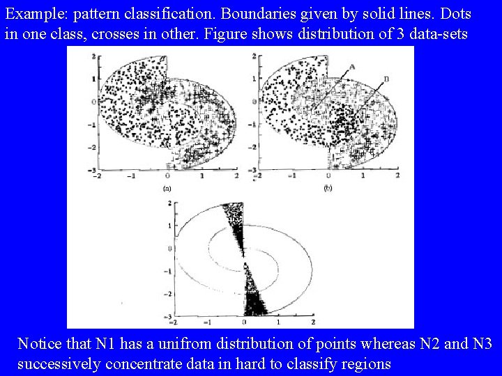
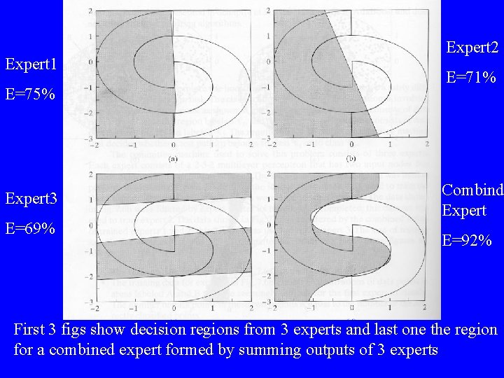
Example: pattern classification. Boundaries given by solid lines. Dots in one class, crosses in other. Figure shows distribution of 3 data-sets Notice that N 1 has a unifrom distribution of points whereas N 2 and N 3 successively concentrate data in hard to classify regions

Expert 1 E=75% Expert 3 E=69% Expert 2 E=71% Combind Expert E=92% First 3 figs show decision regions from 3 experts and last one the region for a combined expert formed by summing outputs of 3 experts

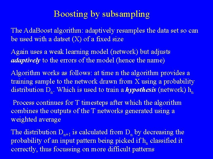
Boosting by subsampling The Ada. Boost algorithm: adaptively resamples the data set so can be used with a datset (X) of a fixed size Again uses a weak learning model (network) but adjusts adaptively to the errors of the model (hence the name) Algorithm works as follows: at time n the algorithm provides a training sample to the network drawn from X using a probability distribution Dn. Which is used to train a hypothesis (network) hn Process continues for T timesteps after which the algorithm combines the outputs of the T networks generated using a weighted average The distribution Dn+1 is calculated from Dn by decreasing the probability of an input pattern being picked if hn classified it correctly, thus focussing on more difficult patterns

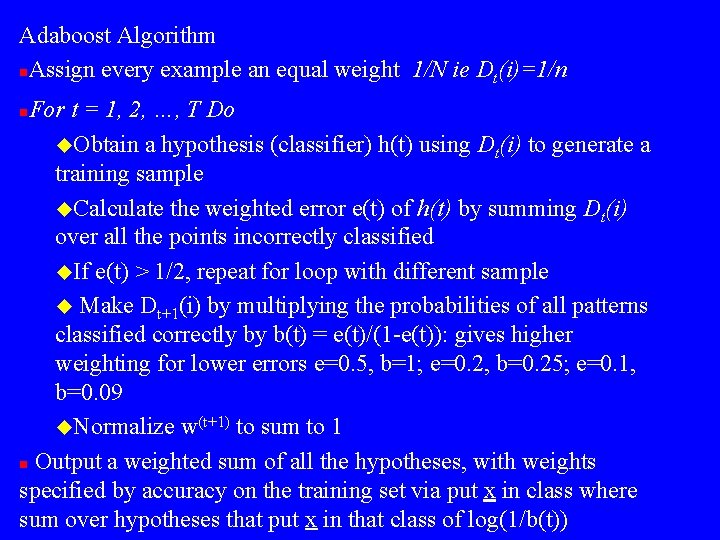
Adaboost Algorithm n. Assign every example an equal weight 1/N ie Dt(i)=1/n For t = 1, 2, …, T Do u. Obtain a hypothesis (classifier) h(t) using Dt(i) to generate a training sample u. Calculate the weighted error e(t) of h(t) by summing Dt(i) over all the points incorrectly classified u. If e(t) > 1/2, repeat for loop with different sample u Make Dt+1(i) by multiplying the probabilities of all patterns classified correctly by b(t) = e(t)/(1 -e(t)): gives higher weighting for lower errors e=0. 5, b=1; e=0. 2, b=0. 25; e=0. 1, b=0. 09 u. Normalize w(t+1) to sum to 1 n Output a weighted sum of all the hypotheses, with weights specified by accuracy on the training set via put x in class where sum over hypotheses that put x in that class of log(1/b(t)) n

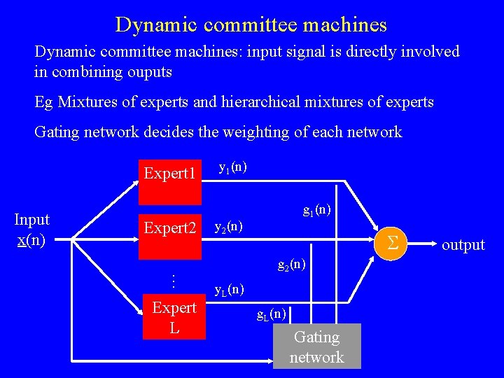
Dynamic committee machines: input signal is directly involved in combining ouputs Eg Mixtures of experts and hierarchical mixtures of experts Gating network decides the weighting of each network Expert 1 Expert 2 … Input x(n) Expert L y 1(n) g 1(n) y 2(n) S g 2(n) y. L(n) g. L(n) Gating network output

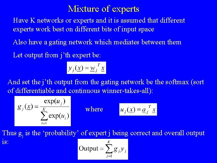
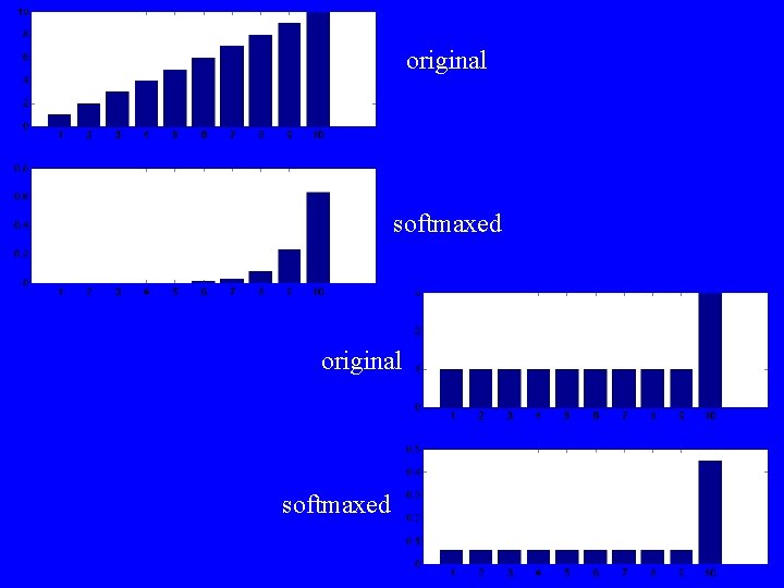
Mixture of experts Have K networks or experts and it is assumed that different experts work best on different bits of input space Also have a gating network which mediates between them Let output from j’th expert be: And set the j’th output from the gating network be the softmax (sort of differentiable and continuous winner-takes-all): where Thus gj is the ‘probability’ of expert j being correct and overall output is:

original softmaxed

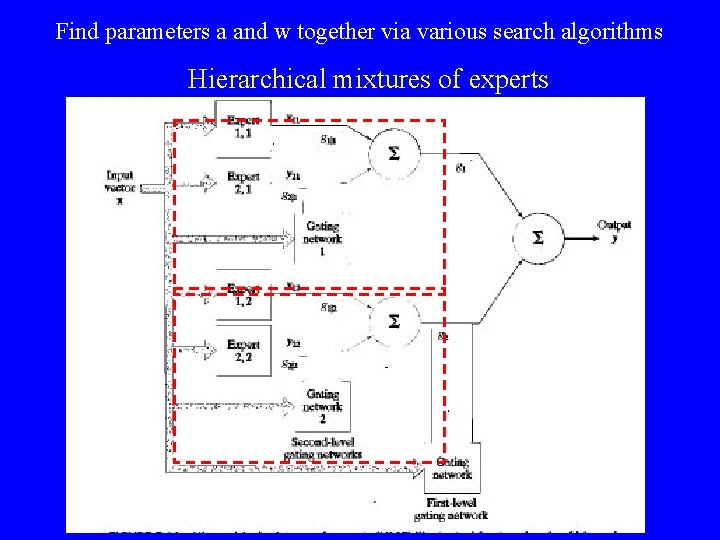
Find parameters a and w together via various search algorithms Hierarchical mixtures of experts