COMMENTS TO Moiras SOME COMMENTS PPT Maxime Le

COMMENTS TO Moira’s SOME COMMENTS. PPT Maxime Le. Goff et Yves Gallet, Institut de Physique du Globe de Paris (France)

1. Why this COMMENTS TO SOME COMMENTS ? We have prepared this slideshow for several reasons: • To answer to the comments sent by M. Wilson after our Quaternary Geochronology (2014) paper. • To answer to the reviewers of our rejected papers (JAS, Archaeometry). • To obtain explanations on the behavior of at least some of the "good" samples studied by the RHX team. • To solve inconsistencies in data interpretation we noted between different publications (Wilson et al. , 2009; 2012 vs. Wilson et al. 2013). • To propose a new way of illustrating the RHX dating results, by using a "timespan analysis“.

Some precisions • The references to Wilson et al, 2009; 2012; 2013 will be often shortened as W 2009; W 2012; W 2013, to Ince’s thesis, 2009 as Ince 2009, and to Le. Goff and Gallet, 2014 as L&G 2014. • From June 2010 until March 2013, we have had several friendly mail exchanges with Moira and Sarah-Jane, sharing some of our respective experiments. • Thanks to her, we received some of their original Xcel workbooks. In particular, we have been able to analyze the series of W 1 and W 2 (weighed from May, 9 th to October 20 th, 2011), sent in August 2012. • Thanks to the use of vectorial graphics format in the Chapter 9 of Ince’s Thesis, we have been able to retrieve four of the series illustrated by her figures 9 -5, 9 -9, 9 -13 and 9 -17. • From June to October 2012, we also tried to perform a comparative test with 5 fragments sent to us by Moira and Sarah-Jane. The unsuccessful results was attributed from an “inadvertently already heated to 500°C” set of fragments. . . • During the past three years, after having constructed and tested a new multi-sample instrument, we have studied more than 150 specimens, from 9 archaeological sites, several times each, resulting in more than 480 weighing series.

2. On the stabilization of sample masses after heating (105°C or 500°C) In all our experiments, we have never reached a satisfactory and trustful mass stability. Each new heating induces various changes in mass level.

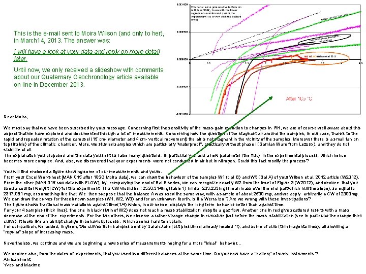
This is the e-mail sent to Moira Wilson (and only to her), in March 14, 2013. The answer was: I will have a look at your data and reply on more detail later. Until now, we only received a slideshow with comments about our Quaternary Geochronology article available on line in December 2013. Dear Moira, We must say that we have been surprised by your message. Concerning first the sensitivity of the mass-gain evolution to changes in RH, we are of course well aware about this aspect that we have explored and documented through a lot of measurements. Concerning now the question of the stagnant air around the samples, in our case, thanks to the rapid and repeated rotation of the carousel (15 cm- diameter and 4 cm- vertical movement) the air is not stagnant in the vicinity of the samples. Moreover there is a small fan on top (inside) of the climatic chamber. More, we studied samples which are particularly "waterproof", practically without phase I (Samian Ware from Lezoux), and they do not stabilize at all. The explanation you proposed and the data you sent us raise many questions. In particular you add a new parameter (the flux) in the experimental process, which hence becomes more complex. And, also, we discovered that your experiments were not conducted in air but in nitrogen. Could this fact modify the process? You will find enclosed a figure showing some of our measurements and yours. From your Excel Worksheet [MAN 015 after 105 C Moira data], we can draw the behaviour of the samples W 1 (bal B) and W 3 (Bal A) of your Wilson et al, 2012 article (W 2012). From the other [MAN 015 raw data with FLOW], by comparying the end of Bal B series, we can recognize exactly W 2 from the inset of Figure 3 (W 2012), and deduce that you used a counter weight (CW) for this experiment. This CW would be : 2550. 314 mg (table 1) minus 233 mg (mean mass over the end part which null the slope), so equal to 2317. 081 mg, or something like that. We then suppose that the balance A was used the same way, with a sample of about 2500 mg, and we apply arbitrarily a CW of 2300 mg. We can draw the curves for three known samples (W 1, W 2, W 3) and for an unknown fourth. Is it a Werra too ? Are we wrong with these investigations? The figure shows fractional mass variations against time(1/4) which, in our sense, displays the long term behavior better than against time. For your 4 samples (thick lines), the one in black (twin of W 2) does not reach a mass stabilization despite a gaz flow. Another one in red give scattered results with a mass decrease at the end of the experiments. For the two others, we observe a rather strange change in curvature just before the mass stabilization (see in particular the orange thick curve). It looks like an abrupt change in behavior/process, which seems hard to explain. For comparison, we added, in green, two curves from samples sent by Sarah Jane (but presumed already heated ? ), and some of ours (thin magenta lines), all showing a "regular" slope of increasing mass. . . Nevertheless, we continue and we are beginning a new series of measurements hoping for a more "ideal" behavior. . . We deduce also, from the dates of experiments, that you used two different balances at the same time. Do you now have a "battery" of such instruments ? Amicalement, Yves and Maxime

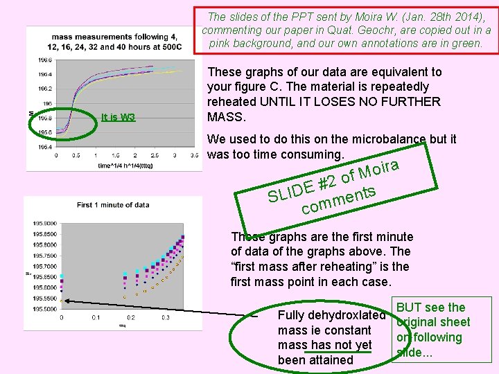
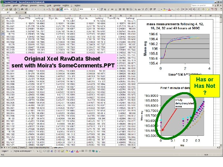
The slides of the PPT sent by Moira W. (Jan. 28 th 2014), commenting our paper in Quat. Geochr, are copied out in a pink background, and our own annotations are in green. It is W 3 These graphs of our data are equivalent to your figure C. The material is repeatedly reheated UNTIL IT LOSES NO FURTHER MASS. We used to do this on the microbalance but it was too time consuming. ira o M of 2 # E SLID mments co These graphs are the first minute of data of the graphs above. The “first mass after reheating” is the first mass point in each case. BUT see the Fully dehydroxlated original sheet mass ie constant on following mass has not yet slide. . . been attained

Original Xcel Raw. Data Sheet sent with Moira's Some. Comments. PPT Has or Has Not ?

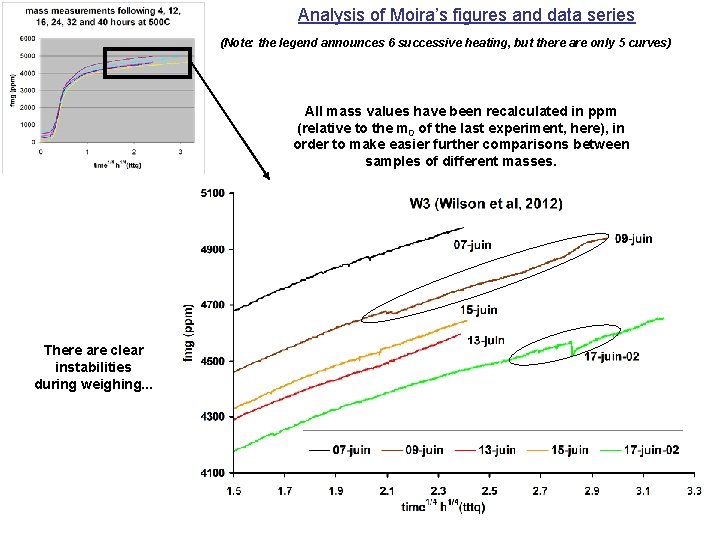
Analysis of Moira’s figures and data series (Note: the legend announces 6 successive heating, but there are only 5 curves) All mass values have been recalculated in ppm (relative to the m 0 of the last experiment, here), in order to make easier further comparisons between samples of different masses. There are clear instabilities during weighing. . .

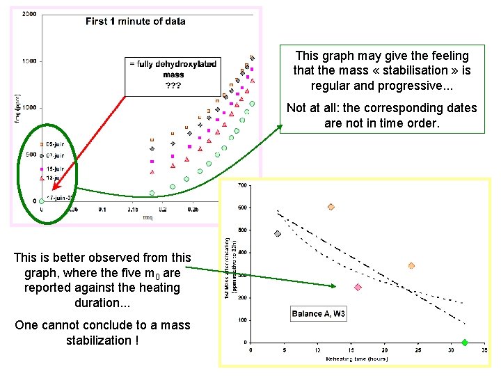
This graph may give the feeling that the mass « stabilisation » is regular and progressive. . . Not at all: the corresponding dates are not in time order. This is better observed from this graph, where the five m 0 are reported against the heating duration. . . One cannot conclude to a mass stabilization !

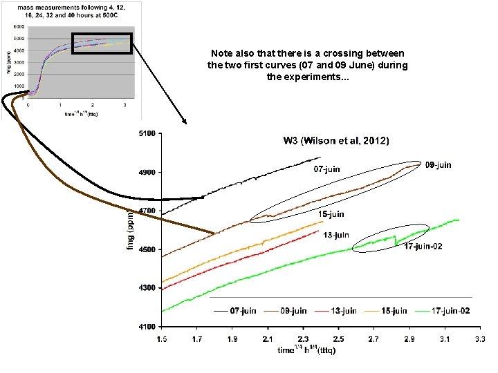
Note also that there is a crossing between the two first curves (07 and 09 June) during the experiments. . .

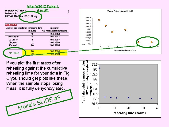
After W 2012 Table 1, it is W 1 If you plot the first mass after reheating against the cumulative reheating time for your data in Fig C you should get plots like these. When the sample stops losing mass, it is fully dehydroxylated, Moi 3 # E ID L S s ra' 1 st data point is mass of clean DRY non-dehydroxylated material No Date 163. 5 163 162. 5 162 161. 5 161 160. 5 160 159. 5 0 10 20 30 reheating time (hours) 40

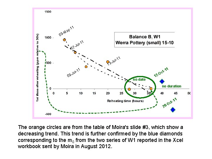
-11 ay M 9 0 11 l-Ju 07 1 l-1 1 u 3 -J 1 t-1 c O 11 l-Ju 09 no date 12 no duration 1 t-1 c O 20 The orange circles are from the table of Moira's slide #3, which show a decreasing trend. This trend is further confirmed by the blue diamonds corresponding to the m 0 from the two series of W 1 reported in the Xcel workbook sent by Moira in August 2012.

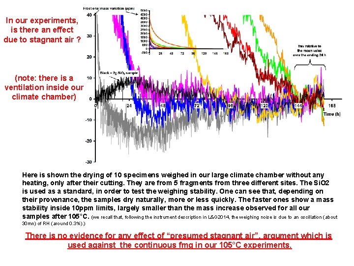
In our experiments, is there an effect due to stagnant air ? (note: there is a ventilation inside our climate chamber) Here is shown the drying of 10 specimens weighed in our large climate chamber without any heating, only after their cutting. They are from 5 fragments from three different sites. The Si. O 2 is used as a standard, in order to test the weighing stability. One can see that, depending on their provenance, the samples dry naturally, more or less quickly. The faster ones show a mass stability inside 10 ppm limits, largely smaller than the mass increase observed for all our samples after 105°C. (we recall that, following the instrument description in L&G 2014, the weighing noise is due to an oscillation (about 30 mn) of RH (around 0. 3%). ) There is no evidence for any effect of “presumed stagnant air”, argument which is used against the continuous fmg in our 105°C experiments.

3. On the stabilization of Rehydroxylation time 1/4 gradient A lot of our specimens fail to provide reliable RHX dating. Despite the explanations provided by Moira, at least some of the good RHX dating results are not reliable.

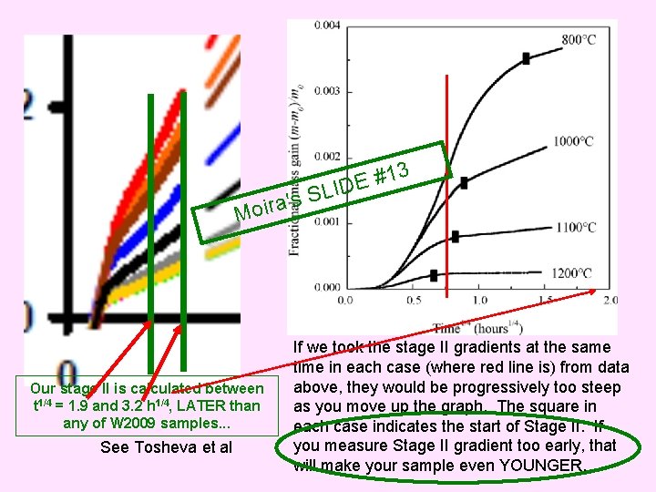
3 a's r i o M Our stage II is calculated between t 1/4 = 1. 9 and 3. 2 h 1/4, LATER than any of W 2009 samples. . . See Tosheva et al 1 # E SLID If we took the stage II gradients at the same time in each case (where red line is) from data above, they would be progressively too steep as you move up the graph. The square in each case indicates the start of Stage II. If you measure Stage II gradient too early, that will make your sample even YOUNGER.

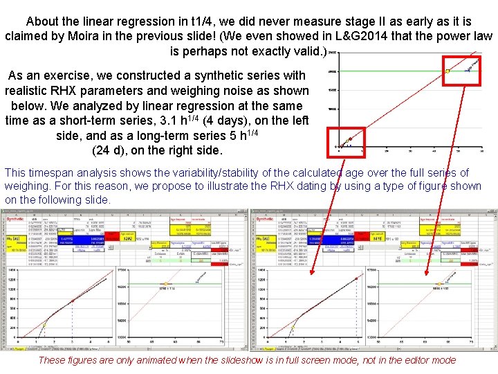
About the linear regression in t 1/4, we did never measure stage II as early as it is claimed by Moira in the previous slide! (We even showed in L&G 2014 that the power law is perhaps not exactly valid. ) As an exercise, we constructed a synthetic series with realistic RHX parameters and weighing noise as shown below. We analyzed by linear regression at the same time as a short-term series, 3. 1 h 1/4 (4 days), on the left side, and as a long-term series 5 h 1/4 (24 d), on the right side. This timespan analysis shows the variability/stability of the calculated age over the full series of weighing. For this reason, we propose to illustrate the RHX dating by using a type of figure shown on the following slide. These figures are only animated when the slideshow is in full screen mode, not in the editor mode

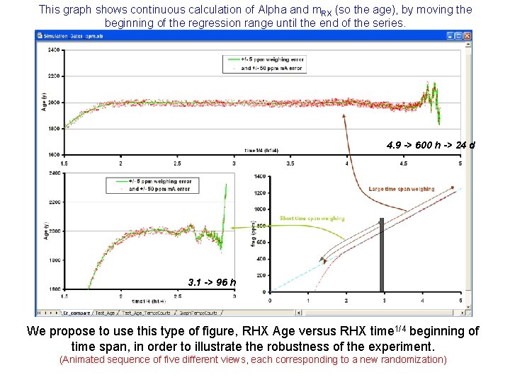
This graph shows continuous calculation of Alpha and m. RX (so the age), by moving the beginning of the regression range until the end of the series. 4. 9 -> 600 h -> 24 d 3. 1 -> 96 h We propose to use this type of figure, RHX Age versus RHX time 1/4 beginning of time span, in order to illustrate the robustness of the experiment. (Animated sequence of five different views, each corresponding to a new randomization)

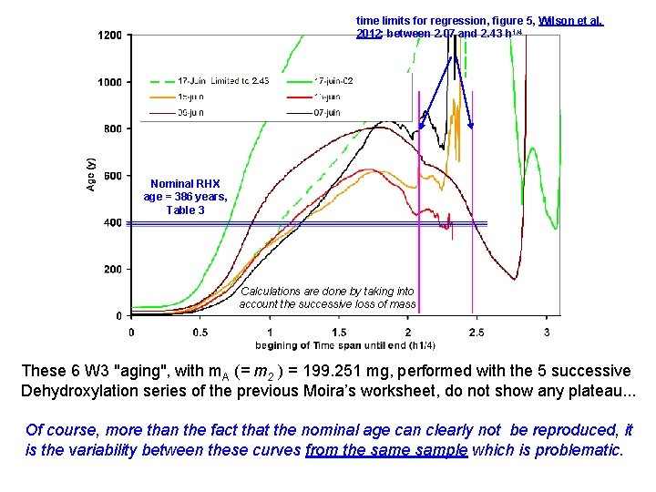
time limits for regression, figure 5, Wilson et al, 2012: between 2. 07 and 2. 43 h 1/4 Nominal RHX age = 386 years, Table 3 Calculations are done by taking into account the successive loss of mass These 6 W 3 "aging", with m. A (= m 2 ) = 199. 251 mg, performed with the 5 successive Dehydroxylation series of the previous Moira’s worksheet, do not show any plateau. . . Of course, more than the fact that the nominal age can clearly not be reproduced, it is the variability between these curves from the sample which is problematic.

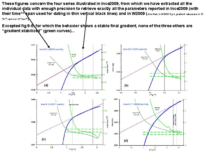
These figures concern the four series illustrated in Ince 2009, from which we have extracted all the individual data with enough precision to retrieve exactly all the parameters reported in Ince 2009 (with their time 1/4 span used for dating in thin vertical black lines) and in W 2009 ( note that, in W 2009 Fig 4, gradient values are in 10 /h , and not 10 /mn ). 4 1/4 -4 1/4 Excepted fig 9 -5, for which the behavior shows a stable final gradient, none of the three others are “gradient stabilized” (green curves). . . -

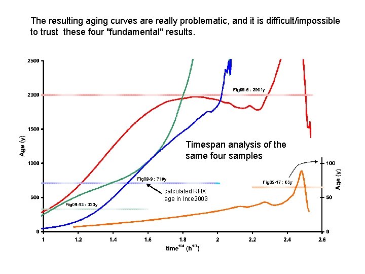
The resulting aging curves are really problematic, and it is difficult/impossible to trust these four "fundamental" results. Timespan analysis of the same four samples calculated RHX age in Ince 2009

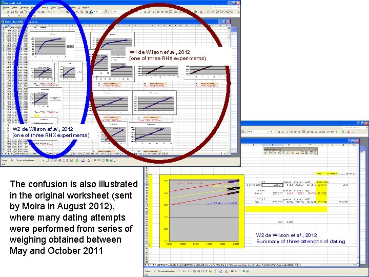
W 1 de Wilson et al. , 2012 (one of three RHX experiments) W 2 de Wilson et al. , 2012 (one of three RHX experiments) The confusion is also illustrated in the original worksheet (sent by Moira in August 2012), where many dating attempts were performed from series of weighing obtained between May and October 2011 W 2 de Wilson et al. , 2012 Summary of three attempts of dating

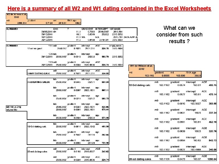
Here is a summary of all W 2 and W 1 dating contained in the Excel Worksheets What can we consider from such results ?

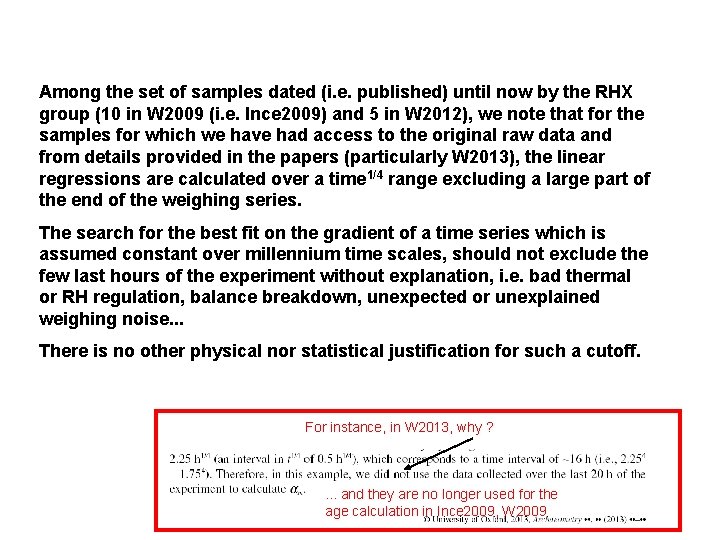
Among the set of samples dated (i. e. published) until now by the RHX group (10 in W 2009 (i. e. Ince 2009) and 5 in W 2012), we note that for the samples for which we have had access to the original raw data and from details provided in the papers (particularly W 2013), the linear regressions are calculated over a time 1/4 range excluding a large part of the end of the weighing series. The search for the best fit on the gradient of a time series which is assumed constant over millennium time scales, should not exclude the few last hours of the experiment without explanation, i. e. bad thermal or RH regulation, balance breakdown, unexpected or unexplained weighing noise. . . There is no other physical nor statistical justification for such a cutoff. For instance, in W 2013, why ? . . . and they are no longer used for the age calculation in Ince 2009, W 2009

4. On the Specific Surface Area (SSA) (and comments on W 2013)

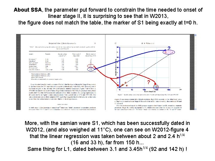
About SSA, the parameter put forward to constrain the time needed to onset of linear stage II, it is surprising to see that in W 2013, the figure does not match the table, the marker of S 1 being exactly at t=0 h. ? ? More, with the samian ware S 1, which has been successfully dated in W 2012, (and also weighed at 11°C), one can see on W 2012 -figure 4 that the linear regression was taken between about 2 and 2. 4 h 1/4 (16 and 33 h), far from 150 h. . . Same thing for L 1, dated between 3. 1 and 3. 45 h 1/4 (92 and 142 h) !

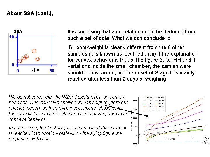
About SSA (cont. ), It is surprising that a correlation could be deduced from such a set of data. What we can conclude is: SSA t (h) i) Loom-weight is clearly different from the 6 other samples (it is known as low-fired. . . ); ii) If the explanation for convex behavior is that of the figure 6, i. e. HR and T variations inside the small chamber, the samian ware should be discarded; iii) The onset of Stage II is mainly reached after less than 2 days of weighing. We do not agree with the W 2013 explanation on convex behavior. This is that we showed with this figure (from our rejected paper), with 10 Syrian specimens, showing, in the exactly the same climate condition, convex, normal or concave behavior. In our opinion, the best way to be convinced that Stage II is reached is to obtain a plateau on the aging figure we propose now to use.

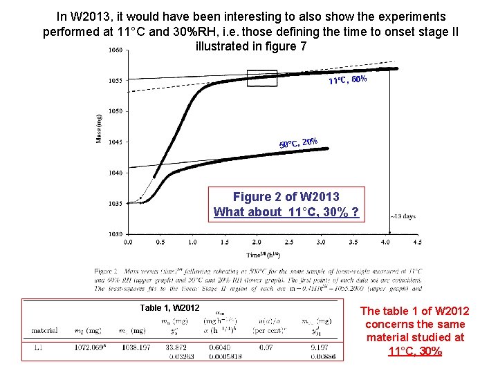
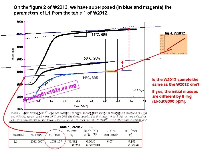
In W 2013, it would have been interesting to also show the experiments performed at 11°C and 30%RH, i. e. those defining the time to onset stage II illustrated in figure 7 11°C, 60% % 50°C, 20 Figure 2 of W 2013 What about 11°C, 30% ? Table 1, W 2012 The table 1 of W 2012 concerns the same material studied at 11°C, 30%

On the figure 2 of W 2013, we have superposed (in blue and magenta) the parameters of L 1 from the table 1 of W 2012. 11°C, 60% fig 4, W 2012 50°C, 20% d se o p p su =1 1 0 m 4 - 11°C, 30% g 0 m 0. 9 02 m Table 1, W 2012 Is the W 2013 sample the same as the W 2012 one? If yes, the initial masses are different by 6 mg (about 6000 ppm).

5. On the Effective Lifetime Temperature (ELT) / Energy of Activation (Ea)

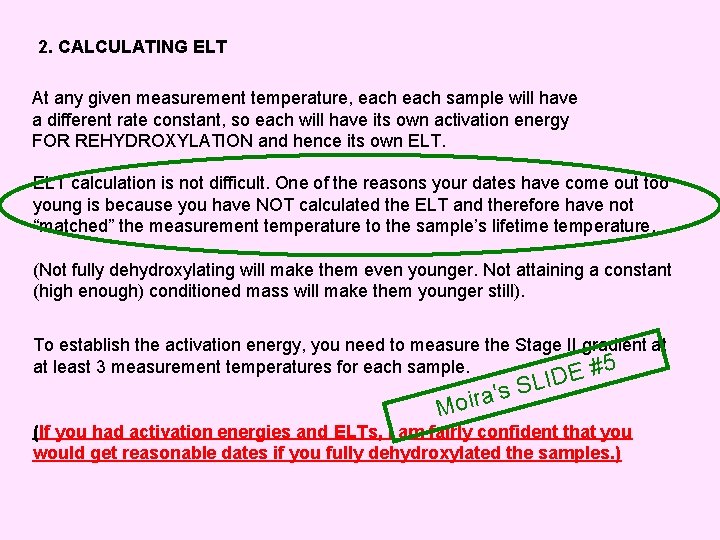
2. CALCULATING ELT At any given measurement temperature, each sample will have a different rate constant, so each will have its own activation energy FOR REHYDROXYLATION and hence its own ELT calculation is not difficult. One of the reasons your dates have come out too young is because you have NOT calculated the ELT and therefore have not “matched” the measurement temperature to the sample’s lifetime temperature. (Not fully dehydroxylating will make them even younger. Not attaining a constant (high enough) conditioned mass will make them younger still). To establish the activation energy, you need to measure the Stage II gradient at at least 3 measurement temperatures for each sample. E #5 M ID L S oira's (If you had activation energies and ELTs, I am fairly confident that you would get reasonable dates if you fully dehydroxylated the samples. )

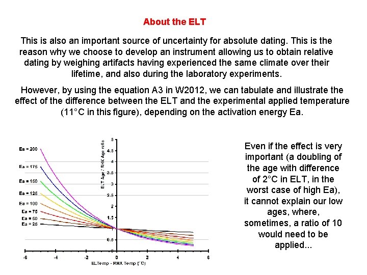
About the ELT This is also an important source of uncertainty for absolute dating. This is the reason why we choose to develop an instrument allowing us to obtain relative dating by weighing artifacts having experienced the same climate over their lifetime, and also during the laboratory experiments. However, by using the equation A 3 in W 2012, we can tabulate and illustrate the effect of the difference between the ELT and the experimental applied temperature (11°C in this figure), depending on the activation energy Ea. Even if the effect is very important (a doubling of the age with difference of 2°C in ELT, in the worst case of high Ea), it cannot explain our low ages, where, sometimes, a ratio of 10 would need to be applied. . .

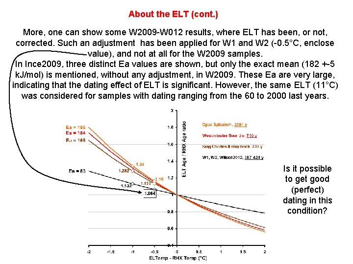
About the ELT (cont. ) More, one can show some W 2009 -W 012 results, where ELT has been, or not, corrected. Such an adjustment has been applied for W 1 and W 2 (-0. 5°C, enclose value), and not at all for the W 2009 samples. In Ince 2009, three distinct Ea values are shown, but only the exact mean (182 +-5 k. J/mol) is mentioned, without any adjustment, in W 2009. These Ea are very large, indicating that the dating effect of ELT is significant. However, the same ELT (11°C) was considered for samples with dating ranging from the 60 to 2000 last years. Is it possible to get good (perfect) dating in this condition?

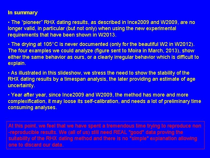
In summary • The “pioneer” RHX dating results, as described in Ince 2009 and W 2009, are no longer valid, in particular (but not only) when using the new experimental requirements that have been shown in W 2013. • The drying at 105°C is never documented (only for the beautiful W 2 in W 2012). The four examples we could analyze (figure sent to Moira in March, 2013), show either the same behavior as ours, or a clearly irregular behavior which is difficult to explain. • As illustrated in this slideshow, we stress the need to show the stability of the RHX dating results by a timespan analysis, the later providing an estimate of age uncertainty. • Year after year, since Ince 2009 and W 2009, the method has more and more complexification, it may loose its self-calibration, and needs a lot of preliminary time consuming analyses. At this point, we feel that we have spent a tremendous time trying to reproduce non -reproducible results. We (all of us) still need REAL "good" data proving the suitability of the RHX dating method and there is no "simple" explanation allowing one to discard our data.