Combining Exact and Heuristic Approaches for the Multidimensional
Combining Exact and Heuristic Approaches for the Multidimensional 0 -1 Knapsack Problem Saïd HANAFI Said. hanafi@univ-valenciennes. fr SYM-OP-IS 2009
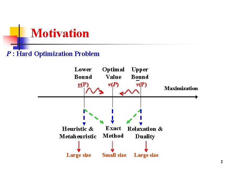
Motivation P : Hard Optimization Problem Lower Bound v(P) Heuristic & Metaheuristic Large size Optimal Value v(P) Upper Bound v(P) Maximization Exact Relaxation & Method Duality Small size Large size 2

Outline n Variants of Multidimensional Knapsack problem (MKP) Tabu Search & Dynamic Programming Relaxations of MKP Iterative Relaxation-based Heuristics n Inequalities and Target Objectives n Conclusions n n n 3
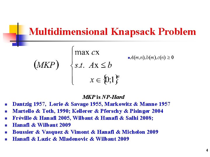
Multidimensional Knapsack Problem n. A(m, n), b(m), c(n) n n n 0 MKP is NP-Hard Dantzig 1957, Lorie & Savage 1955, Markowitz & Manne 1957 Martello & Toth, 1990; Kellerer & Pferschy & Pisinger 2004 Fréville & Hanafi 2005, Wilbaut & Hanafi & Salhi 2008; Hanafi & Wilbaut 2009 Boussier & Vasquez & Vimont & Hanafi & Michelon 2009 Hanafi & Lazic & Mladenovic & Wilbaut 2009 4
Applications n n n n n Resource allocation problems Production scheduling problems Transportation management problems Adaptive multimedia system with Qo. S Telecommunication networks problems Wireless switch design Service selection for web services with Qo. S constraints Polyedral approach, (1, k)-configuration Sub-problem : Lagrangean / Surrogate relaxation Benchmark 5
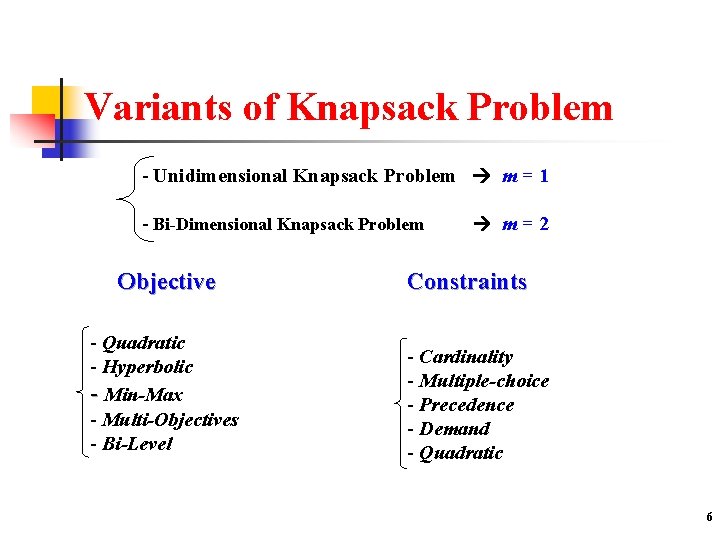
Variants of Knapsack Problem - Unidimensional Knapsack Problem m = 1 - Bi-Dimensional Knapsack Problem m = 2 Objective - Quadratic - Hyperbolic - Min-Max - Multi-Objectives - Bi-Level Constraints - Cardinality - Multiple-choice - Precedence - Demand - Quadratic 6
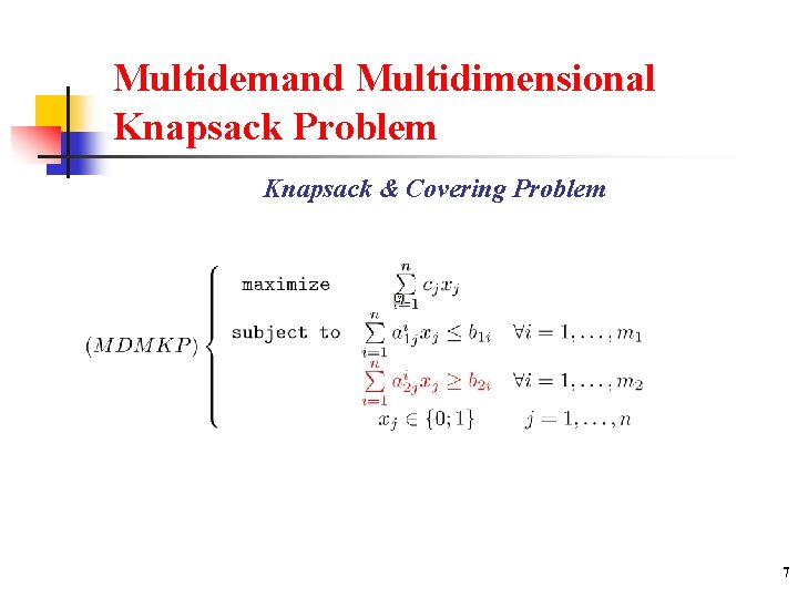
Multidemand Multidimensional Knapsack Problem Knapsack & Covering Problem 7
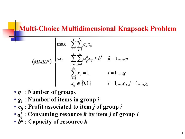
Multi-Choice Multidimensional Knapsack Problem • g : Number of groups • gi : Number of items in group i • cij : Profit associated to item j of group i • : Consuming resource k by item j of group i • bk : Capacity of resource k 8
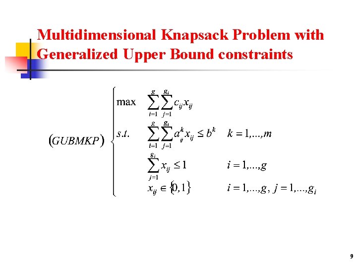
Multidimensional Knapsack Problem with Generalized Upper Bound constraints 9
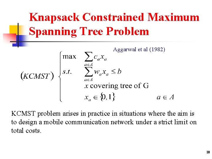
Knapsack Constrained Maximum Spanning Tree Problem Aggarwal et al (1982) KCMST problem arises in practice in situations where the aim is to design a mobile communication network under a strict limit on total costs. 10
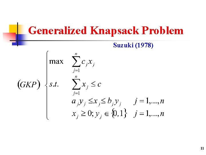
Generalized Knapsack Problem Suzuki (1978) 11
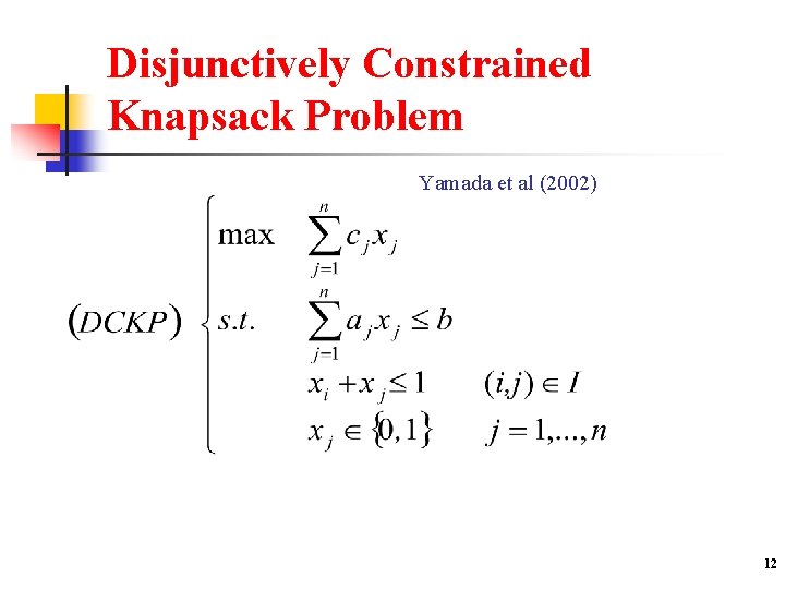
Disjunctively Constrained Knapsack Problem Yamada et al (2002) 12
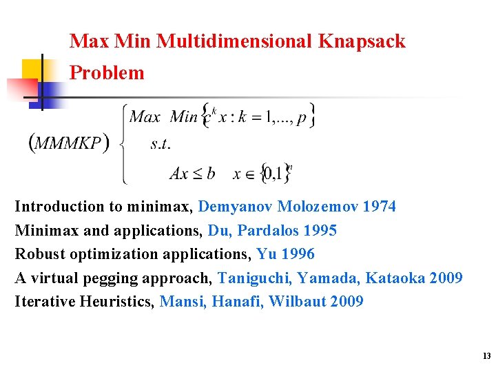
Max Min Multidimensional Knapsack Problem Introduction to minimax, Demyanov Molozemov 1974 Minimax and applications, Du, Pardalos 1995 Robust optimization applications, Yu 1996 A virtual pegging approach, Taniguchi, Yamada, Kataoka 2009 Iterative Heuristics, Mansi, Hanafi, Wilbaut 2009 13
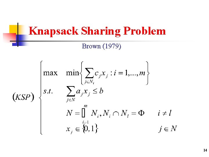
Knapsack Sharing Problem Brown (1979) 14
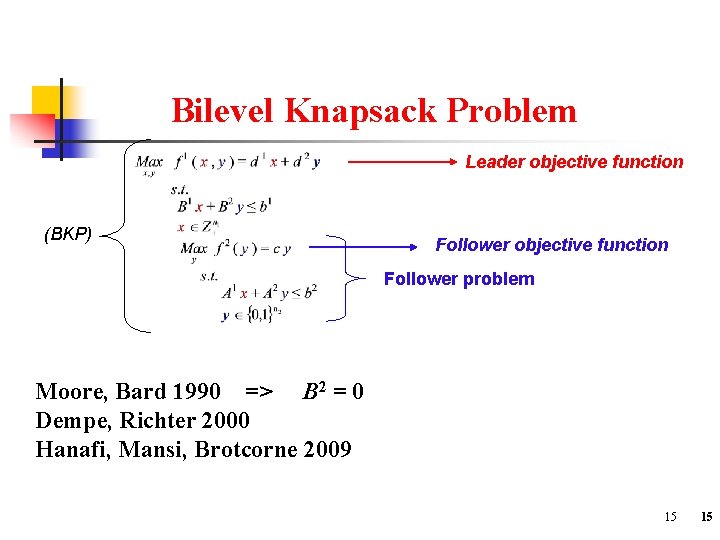
Bilevel Knapsack Problem Leader objective function (BKP) Follower objective function Follower problem Moore, Bard 1990 => B 2 = 0 Dempe, Richter 2000 Hanafi, Mansi, Brotcorne 2009 15 15
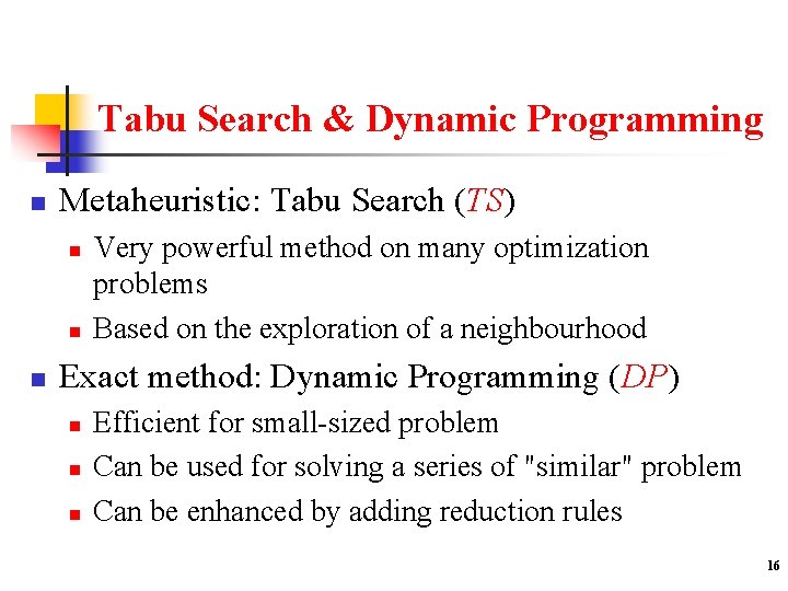
Tabu Search & Dynamic Programming n Metaheuristic: Tabu Search (TS) n n n Very powerful method on many optimization problems Based on the exploration of a neighbourhood Exact method: Dynamic Programming (DP) n n n Efficient for small-sized problem Can be used for solving a series of "similar" problem Can be enhanced by adding reduction rules 16
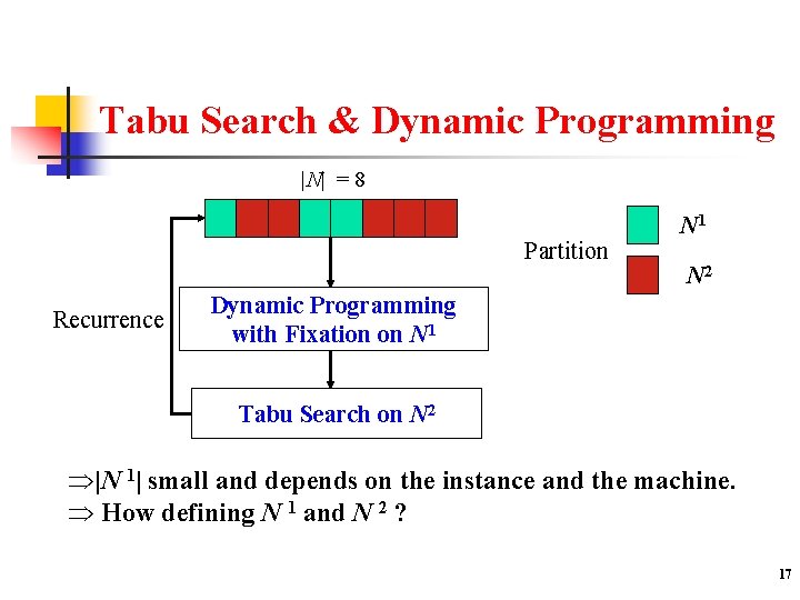
Tabu Search & Dynamic Programming |N| = 8 Partition Recurrence N 1 N 2 Dynamic Programming with Fixation on N 1 Tabu Search on N 2 |N 1| small and depends on the instance and the machine. How defining N 1 and N 2 ? 17
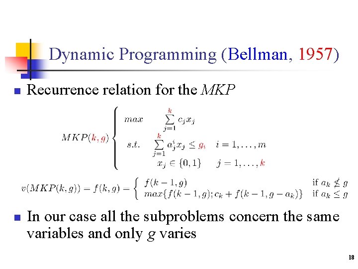
Dynamic Programming (Bellman, 1957) n n Recurrence relation for the MKP In our case all the subproblems concern the same variables and only g varies 18

Reduction Rules n Let x 0 be a feasible solution of the MKP. Order the variables such that: n n n Proposition 1 (Optimality): Let n , Proposition 2 (Fixation): Balev, Fréville, Yanev and Andonov, 2001. 19
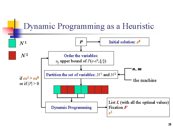
Dynamic Programming as a Heuristic N 1 N 2 P Initial solution: x 0 Order the variables: uj upper bound of P(e-x 0, {j}) n, m if cx 1 > cx 0 or if |F| > 0 Partition the set of variables: N 1 and N 2 the machine Dynamic Programming List L (with all the optimal values) Fixation F x 1 20
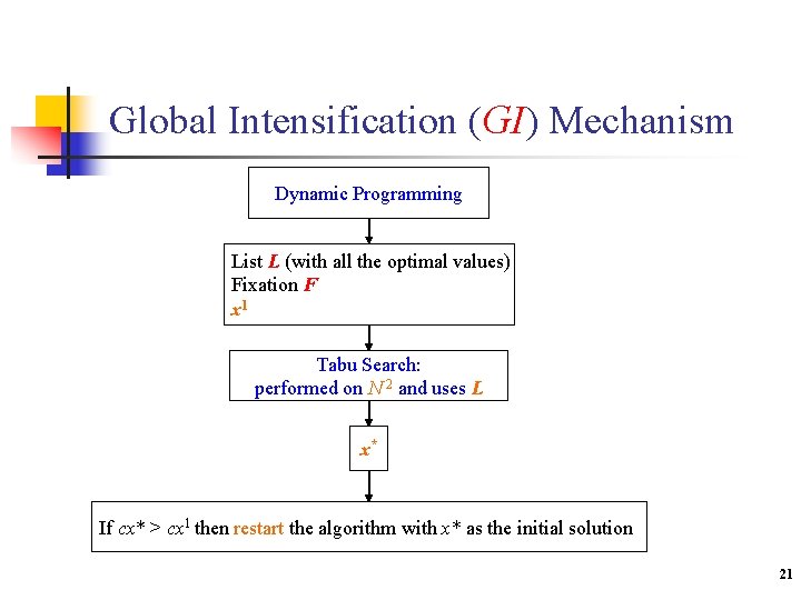
Global Intensification (GI) Mechanism Dynamic Programming List L (with all the optimal values) Fixation F x 1 Tabu Search: performed on N 2 and uses L x* If cx* > cx 1 then restart the algorithm with x* as the initial solution 21
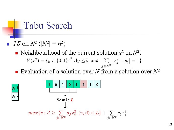
Tabu Search n TS on N 2 (|N 2| = n 2) n Neighbourhood of the current solution x 2 on N 2: n Evaluation of a solution over N from a solution over N 2 N 1 N 2 1? 0 1 ? 0 ? 1 1 0 Scan in L 22
Computational Environment n n Algorithm coded in C language The results have been obtained on a Solaris Ultra Sparc workstation 300 MHz n 1 15% of n OR-Library : 270 correlated instances n n n = 100, 250, 500 and m = 5, 10, 30 30 instances for each (n, m) 23
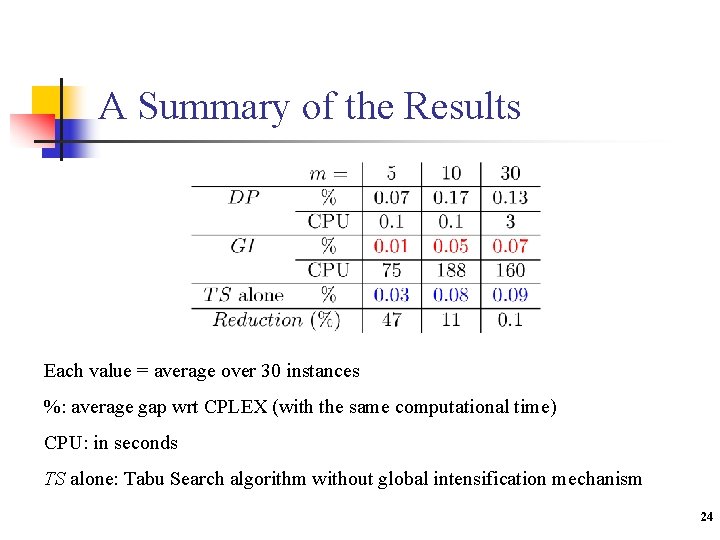
A Summary of the Results Each value = average over 30 instances %: average gap wrt CPLEX (with the same computational time) CPU: in seconds TS alone: Tabu Search algorithm without global intensification mechanism 24

Relaxation Definition : Let (P) max{ f(x) : x X} (R) max{ g(x) : x Y} Problem R is a relaxation of P if 1) X Y 2) x X : f(x) ≤ g(x). Properties - v(P) ≤ v(R) - Let x* an optimal solution of R, if x* is feasible for P and f(x*)=g(x*) then x* is an optimal solution of P 25
![LP-Relaxation Dantzig (1957) (LP) max cx s. t. Ax ≤ b x [0, 1]n LP-Relaxation Dantzig (1957) (LP) max cx s. t. Ax ≤ b x [0, 1]n](http://slidetodoc.com/presentation_image/19282fd749a1c6e4da68d487a4e319fd/image-26.jpg)
LP-Relaxation Dantzig (1957) (LP) max cx s. t. Ax ≤ b x [0, 1]n Properties : - v(MKP) ≤ v(LP) - Let x* an optimal solution of LP, if x* {0, 1}n then x* is an optimal solution of MKP 26

MIP Relaxation Hanafi & Wilbaut (06), Glover (06) n Let x 0 {0, 1}n and J N n Remarks: n n n MIP(x 0, ) = LP(P), MIP(x 0, N) = P v(MIP(x 0, J)) v(MIP(x 0, J’) if J J’ Stronger bound : v(P) v(MIP(P, J)) v(LP(P)) 27

Lagrangean Relaxation Held & Krap (71), Geoffrion (74) n n Lagrangean Relaxation : 0 LR( ) max{cx + (b – Ax) : x X} Lagrangean Dual : (L) min{v(LR( )) : 0} Properties : - v(MKP) ≤ v(LR( )) - Let x* be an optimal solution of LR( *), if *(b – Ax*) = 0 and x* is feasible for P then x* is an optimal solution of P 28
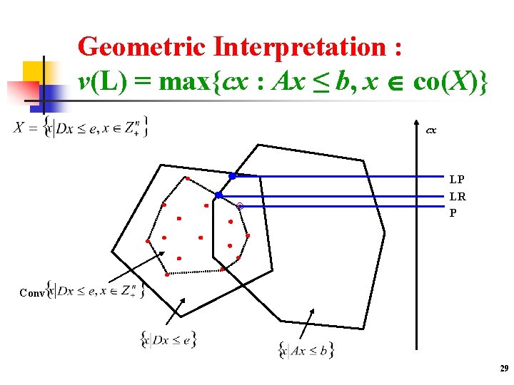
Geometric Interpretation : v(L) = max{cx : Ax ≤ b, x co(X)} cx LP LR P Conv 29
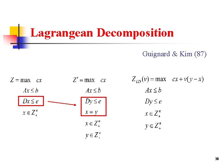
Lagrangean Decomposition Guignard & Kim (87) 30
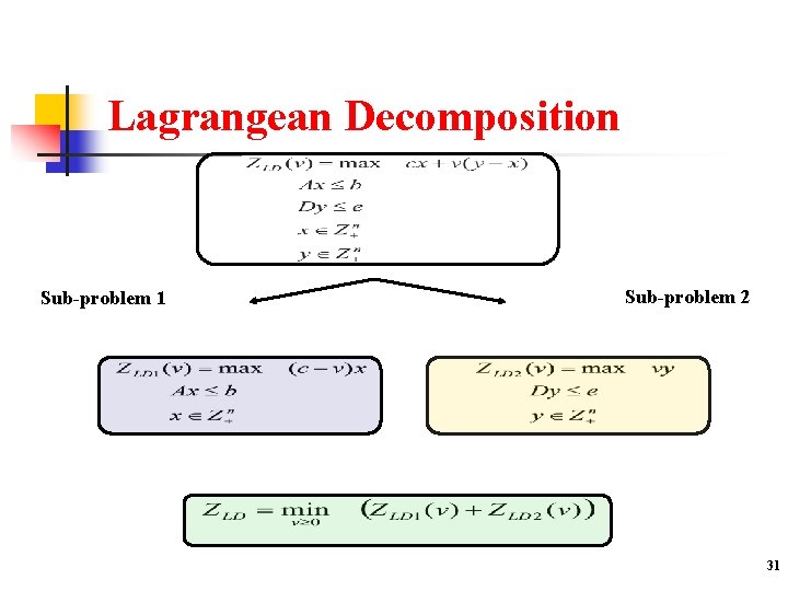
Lagrangean Decomposition Sub-problem 1 Sub-problem 2 31
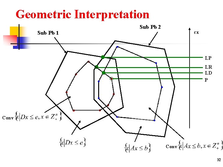
Geometric Interpretation Sub Pb 1 Sub Pb 2 cx LP LR LD P Conv 32
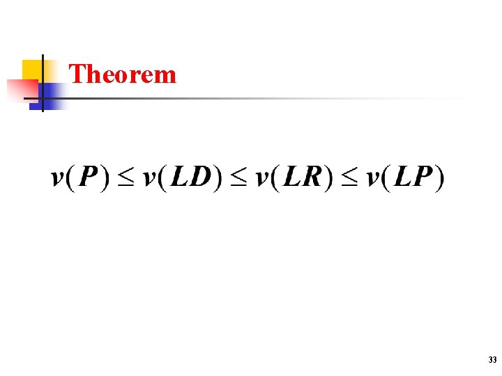
Theorem 33
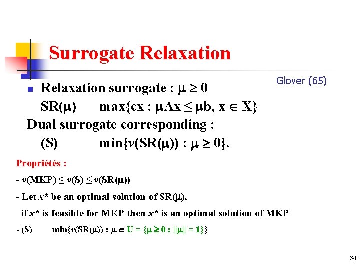
Surrogate Relaxation surrogate : 0 SR( ) max{cx : Ax ≤ b, x X} Dual surrogate corresponding : (S) min{v(SR( )) : 0}. n Glover (65) Propriétés : - v(MKP) ≤ v(SR( )) - Let x* be an optimal solution of SR( ), if x* is feasible for MKP then x* is an optimal solution of MKP - (S) min{v(SR( )) : U = { 0 : || || = 1}} 34
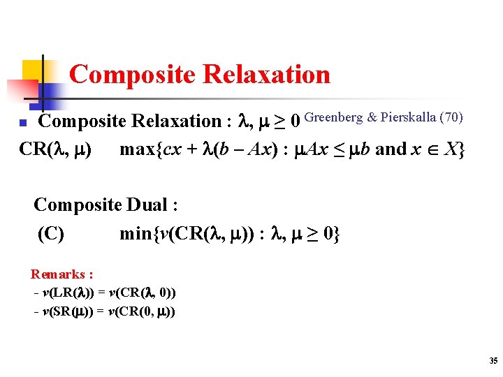
Composite Relaxation : , ≥ 0 Greenberg & Pierskalla (70) CR( , ) max{cx + (b – Ax) : Ax ≤ b and x X} n Composite Dual : (C) min{v(CR( , )) : , ≥ 0} Remarks : - v(LR( )) = v(CR( , 0)) - v(SR( )) = v(CR(0, )) 35

Comparisons v(P) v(C) v(S) v(LP) 36
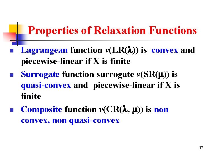
Properties of Relaxation Functions n n n Lagrangean function v(LR( )) is convex and piecewise-linear if X is finite Surrogate function surrogate v(SR( )) is quasi-convex and piecewise-linear if X is finite Composite function v(CR( , )) is non convex, non quasi-convex 37
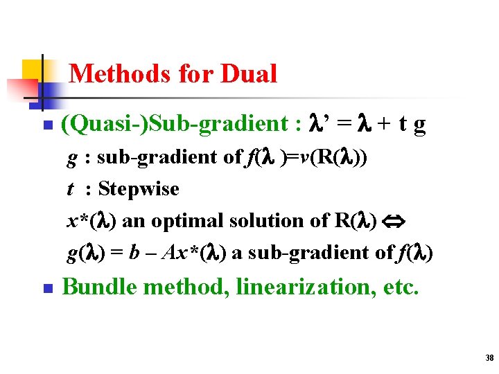
Methods for Dual n (Quasi-)Sub-gradient : ’ = + t g g : sub-gradient of f( )=v(R( )) t : Stepwise x*( ) an optimal solution of R( ) g( ) = b – Ax*( ) a sub-gradient of f( ) n Bundle method, linearization, etc. 38
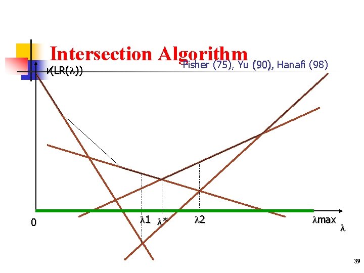
Intersection Algorithm Fisher (75), Yu (90), Hanafi (98) v(LR( )) 0 1 * 2 max 39
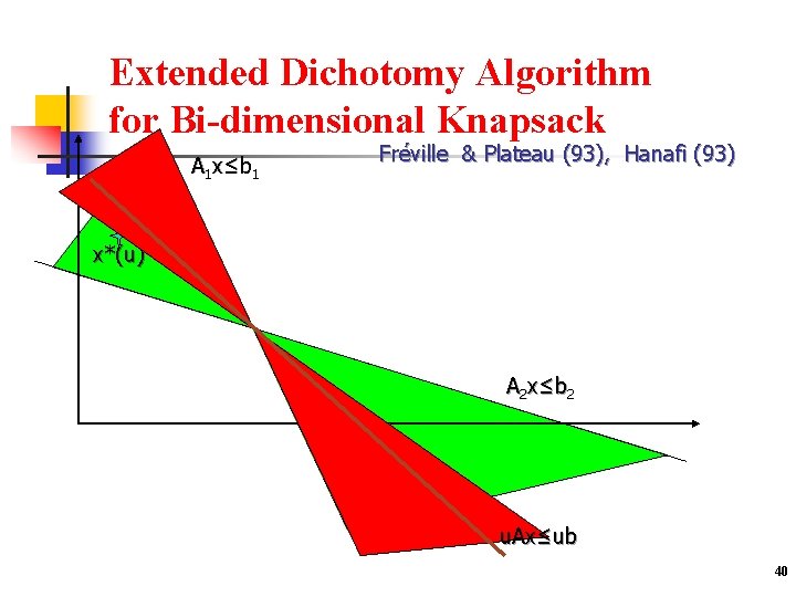
Extended Dichotomy Algorithm for Bi-dimensional Knapsack A 1 x≤ b 1 Fréville & Plateau (93), Hanafi (93) x*(u) A 2 x≤ b 2 u. Ax≤ub 40
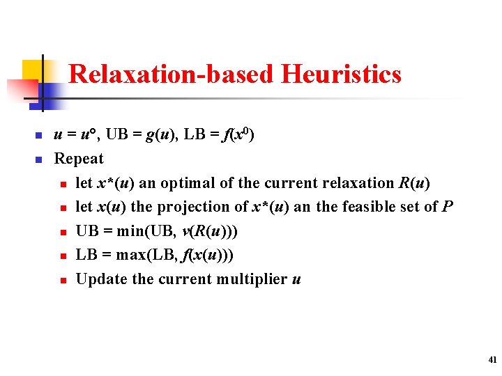
Relaxation-based Heuristics n n u = u°, UB = g(u), LB = f(x 0) Repeat n let x*(u) an optimal of the current relaxation R(u) n let x(u) the projection of x*(u) an the feasible set of P n UB = min(UB, v(R(u))) n LB = max(LB, f(x(u))) n Update the current multiplier u 41
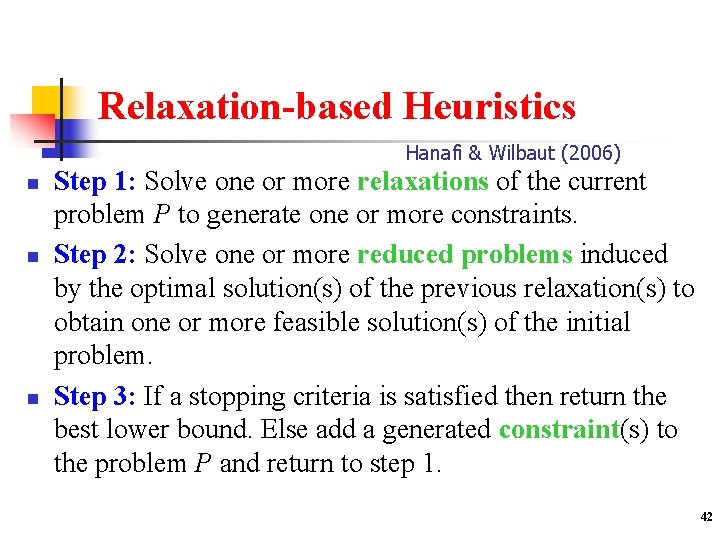
Relaxation-based Heuristics Hanafi & Wilbaut (2006) n n n Step 1: Solve one or more relaxations of the current problem P to generate one or more constraints. Step 2: Solve one or more reduced problems induced by the optimal solution(s) of the previous relaxation(s) to obtain one or more feasible solution(s) of the initial problem. Step 3: If a stopping criteria is satisfied then return the best lower bound. Else add a generated constraint(s) to the problem P and return to step 1. 42
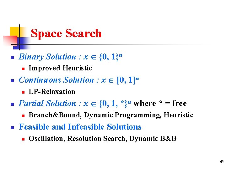
Space Search n Binary Solution : x {0, 1}n n n Continuous Solution : x [0, 1]n n n LP-Relaxation Partial Solution : x {0, 1, *}n where * = free n n Improved Heuristic Branch&Bound, Dynamic Programming, Heuristic Feasible and Infeasible Solutions n Oscillation, Resolution Search, Dynamic B&B 43
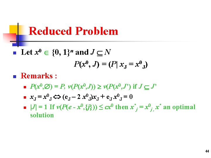
Reduced Problem n n Let x 0 {0, 1}n and J N P(x 0, J) = (P| x. J = x 0 J) Remarks : n n n P(x 0, ) = P, v(P(x 0, J)) v(P(x 0, J’) if J J’ x. J = x 0 J (e. J – 2 x 0 J)x. J + e. J x 0 J = 0 |J| = 1 If v(P(e - x 0, {j})) ≤ cx 0 then x*j = x 0 j , x* an optimal solution 44

LP-based Heuristic n Step 1: Solve the LP-relaxation of P to obtain an optimal solution x. LP Step 2: Solve the reduced problem P(x. LP, J(x. LP)) to generate an optimal solution x 0 where J (x) = {j N : xj {0, 1}} n Remarks: n n n cx 0 ≤ v(P) ≤ cx. LP Relaxation induced neighbourhoods search, Danna et al. , 2003 P((x. LP+x*)/2, J((x. LP+x*))/2) with cx > cx* where x* the best feasible solution 45
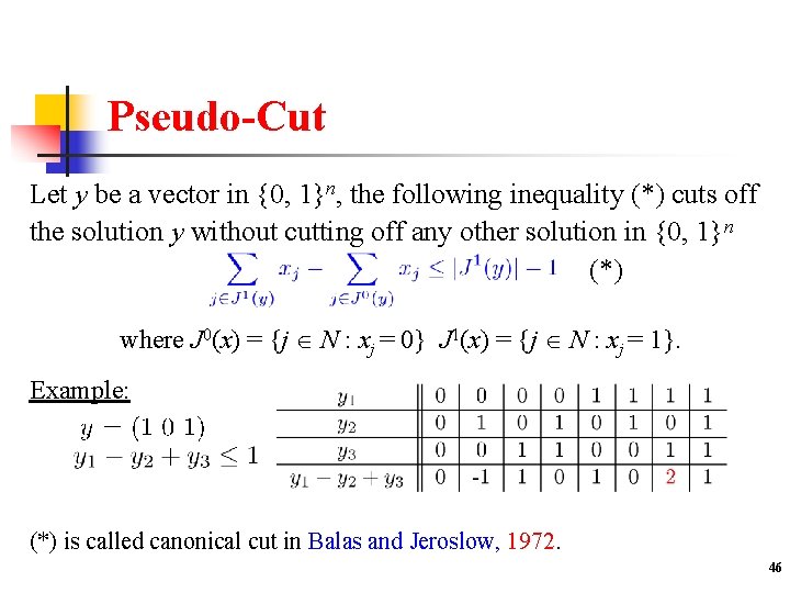
Pseudo-Cut Let y be a vector in {0, 1}n, the following inequality (*) cuts off the solution y without cutting off any other solution in {0, 1}n (*) where J 0(x) = {j N : xj = 0} J 1(x) = {j N : xj = 1}. Example: (*) is called canonical cut in Balas and Jeroslow, 1972. 46
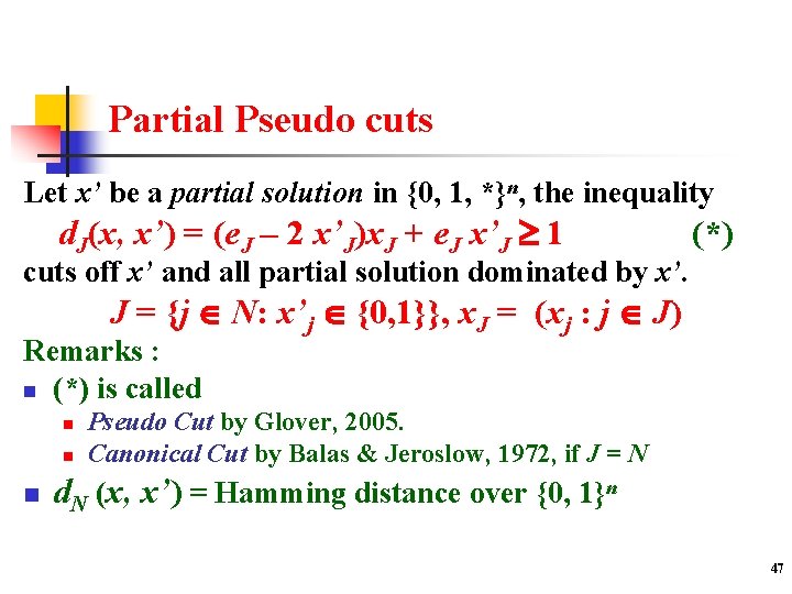
Partial Pseudo cuts Let x’ be a partial solution in {0, 1, *}n, the inequality d. J(x, x’) = (e. J – 2 x’J)x. J + e. J x’J 1 (*) cuts off x’ and all partial solution dominated by x’. J = {j N: x’j {0, 1}}, x. J = (xj : j J) Remarks : n (*) is called n n n Pseudo Cut by Glover, 2005. Canonical Cut by Balas & Jeroslow, 1972, if J = N d. N (x, x’) = Hamming distance over {0, 1}n 47
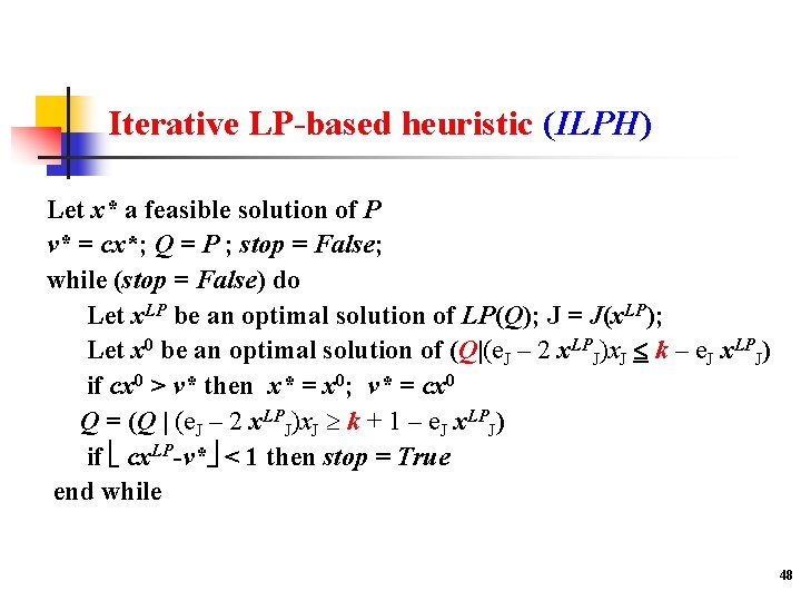
Iterative LP-based heuristic (ILPH) Let x* a feasible solution of P v* = cx*; Q = P ; stop = False; while (stop = False) do Let x. LP be an optimal solution of LP(Q); J = J(x. LP); Let x 0 be an optimal solution of (Q|(e. J – 2 x. LPJ)x. J k – e. J x. LPJ) if cx 0 > v* then x* = x 0; v* = cx 0 Q = (Q | (e. J – 2 x. LPJ)x. J k + 1 – e. J x. LPJ) if cx. LP-v* < 1 then stop = True end while 48
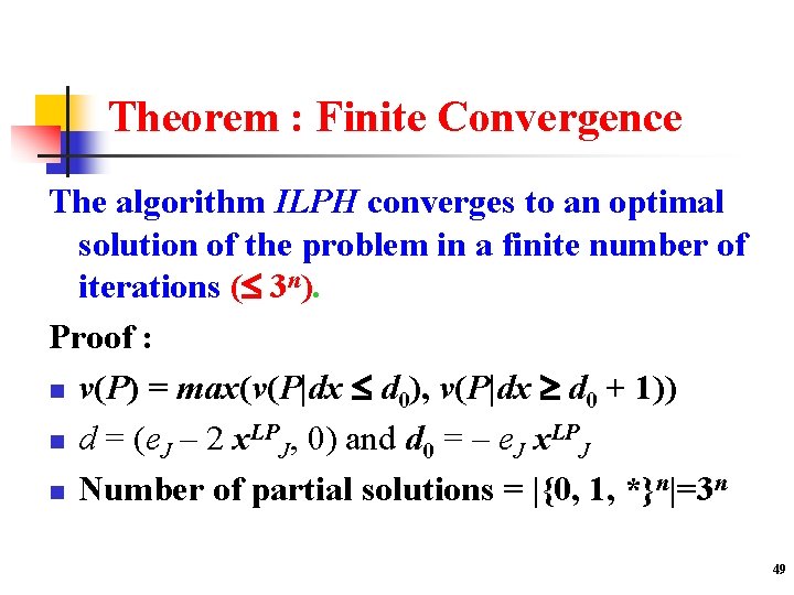
Theorem : Finite Convergence The algorithm ILPH converges to an optimal solution of the problem in a finite number of iterations ( 3 n). Proof : n v(P) = max(v(P|dx d 0), v(P|dx d 0 + 1)) n d = (e. J – 2 x. LPJ, 0) and d 0 = – e. J x. LPJ n Number of partial solutions = |{0, 1, *}n|=3 n 49
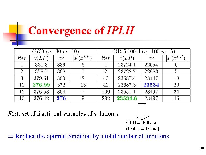
Convergence of IPLH F(x): set of fractional variables of solution x CPU 400 sec (Cplex 10 sec) Replace the optimal condition by a total number of iterations 50
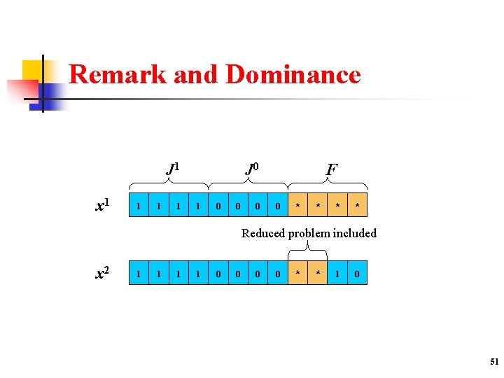
Remark and Dominance J 1 x 1 1 J 0 1 0 0 0 F 0 * * Reduced problem included x 2 1 1 0 0 * * 1 0 51

Improvements: Dominance Properties Definition: Let x 1 and x 2 be two solutions in [0, 1]n, x 1 dominates x 2 if F(x 2) F(x 1), J 1(x 1) J 1(x 2) and J 0(x 1) J 0(x 2) Property 1: If x 1 dominates x 2 then v(P(x 1, J(x 1))) v(P(x 2, J(x 2))) Property 2: The solution x defined by dominates x 1 and x 2, and we have : v(P(x, J(x))) max { v(P(x 1, J(x 1))) , v(P(x 2, J(x 2))) } Reduction of the number of reduced problems to solve 52
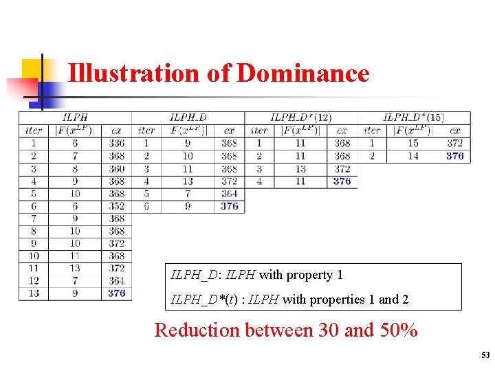
Illustration of Dominance ILPH_D: ILPH with property 1 ILPH_D*(t) : ILPH with properties 1 and 2 Reduction between 30 and 50% 53

Iterative independent relaxations-based heuristic (IIRH) Q = P, x 0 optimal solution of LP(P); k = 1 yk optimal solution of LP(Pk) wk optimal solution of P(yk, J(yk)) xk optimal solution of MIP(Qk, F(xk-1)) zk optimal solution of Q(xk, J(xk)) v*= max(v*, cwk, czk) u = min(cyk, cxk) Pk+1 = (Pk | {f kx ≤ | J 1(yk)| - 1} k=k+1 No Q k+1 = (Q k | {f kx ≤ | J 1(xk)| - 1} If u –v*< 1 Yes Stop 54
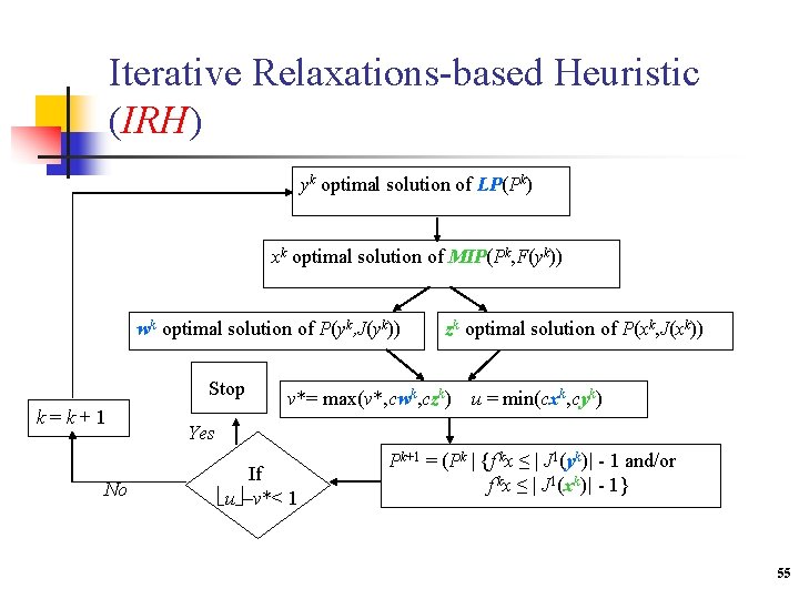
Iterative Relaxations-based Heuristic (IRH) yk optimal solution of LP(Pk) xk optimal solution of MIP(Pk, F(yk)) wk optimal solution of P(yk, J(yk)) Stop k=k+1 No zk optimal solution of P(xk, J(xk)) v*= max(v*, cwk, czk) u = min(cxk, cyk) Yes If u –v*< 1 Pk+1 = (Pk | {f kx ≤ | J 1(yk)| - 1 and/or f kx ≤ | J 1(xk)| - 1} 55
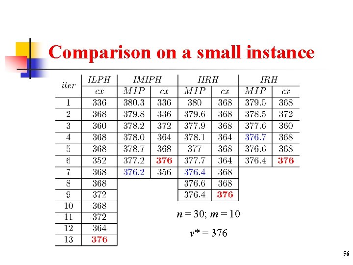
Comparison on a small instance n = 30; m = 10 v* = 376 56
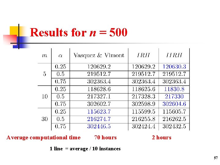
Results for n = 500 Average computational time 70 hours 2 hours 1 line = average / 10 instances 57
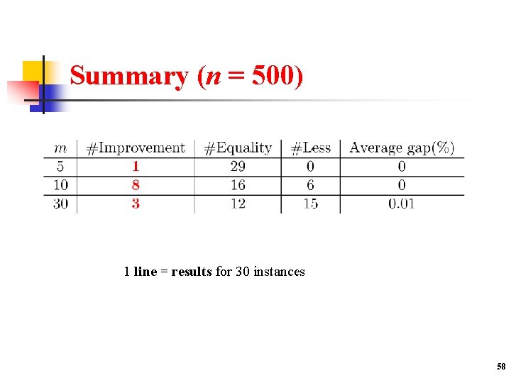
Summary (n = 500) 1 line = results for 30 instances 58
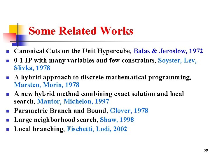
Some Related Works n n n n Canonical Cuts on the Unit Hypercube, Balas & Jeroslow, 1972 0 -1 IP with many variables and few constraints, Soyster, Lev, Slivka, 1978 A hybrid approach to discrete mathematical programming, Marsten, Morin, 1978 A new hybrid method combining exact solution and local search, Mautor, Michelon, 1997 Parametric Branch and Bound, Glover, 1978 Large neighborhood search, Shaw, 1998 Local branching, Fischetti, Lodi, 2002 59
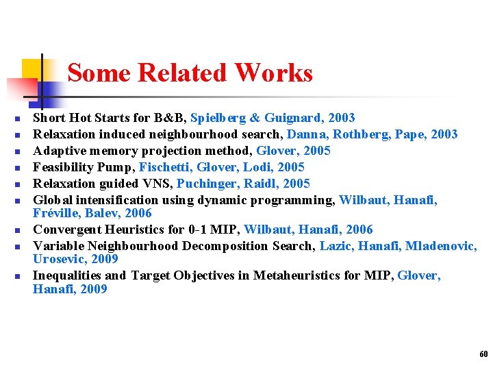
Some Related Works n n n n n Short Hot Starts for B&B, Spielberg & Guignard, 2003 Relaxation induced neighbourhood search, Danna, Rothberg, Pape, 2003 Adaptive memory projection method, Glover, 2005 Feasibility Pump, Fischetti, Glover, Lodi, 2005 Relaxation guided VNS, Puchinger, Raidl, 2005 Global intensification using dynamic programming, Wilbaut, Hanafi, Fréville, Balev, 2006 Convergent Heuristics for 0 -1 MIP, Wilbaut, Hanafi, 2006 Variable Neighbourhood Decomposition Search, Lazic, Hanafi, Mladenovic, Urosevic, 2009 Inequalities and Target Objectives in Metaheuristics for MIP, Glover, Hanafi, 2009 60

Inequalities and Target Objectives in Metaheuristics for MIP Glover & Hanafi (09) n n Recent adaptive memory and evolutionary metaheuristics for MIP have included proposals for introducing inequalities and target objectives to guide the search. Two types of search strategies n n Fix subsets of variables to particular values within approaches for exploiting strongly determined and consistent variables, Use of solution targeting procedures. 61
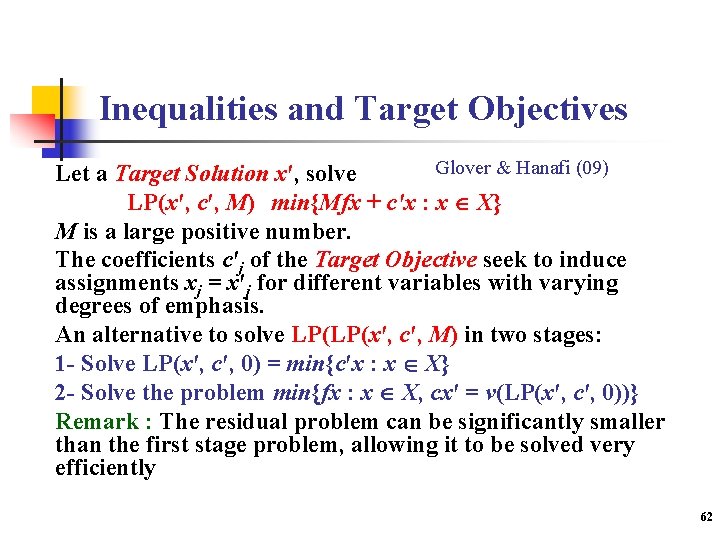
Inequalities and Target Objectives Glover & Hanafi (09) Let a Target Solution x′, solve LP(x′, c′, M) min{Mfx + c′x : x X} M is a large positive number. The coefficients c′j of the Target Objective seek to induce assignments xj = x′j for different variables with varying degrees of emphasis. An alternative to solve LP(LP(x′, c′, M) in two stages: 1 - Solve LP(x′, c′, 0) = min{c′x : x X} 2 - Solve the problem min{fx : x X, cx′ = v(LP(x′, c′, 0))} Remark : The residual problem can be significantly smaller than the first stage problem, allowing it to be solved very efficiently 62
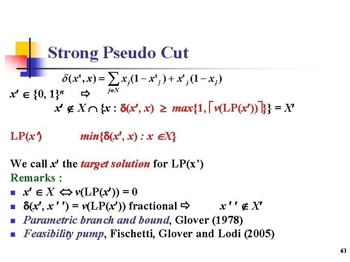
Strong Pseudo Cut x {0, 1}n x X {x : d(x , x) max{1, v(LP(x )) }} = X LP(x ) min{d(x , x) : x X} We call x the target solution for LP(x’) Remarks : n x X v(LP(x )) = 0 n d(x , x ) = v(LP(x )) fractional x X n Parametric branch and bound, Glover (1978) n Feasibility pump, Fischetti, Glover and Lodi (2005) 63
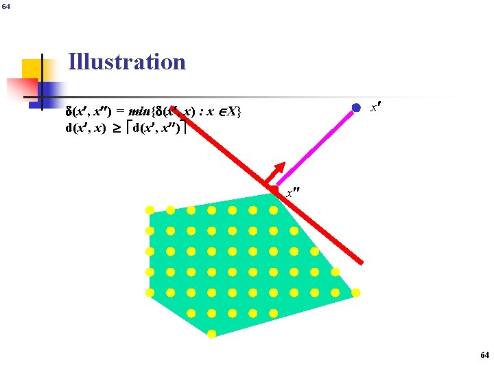
64 Illustration x d(x , x ) = min{d(x , x) : x X} d(x , x) d(x , x ) x Martin Grötschel 64
![Partial Pseudo Cuts Let x [0, 1]n, J N(x ) = {j : xj Partial Pseudo Cuts Let x [0, 1]n, J N(x ) = {j : xj](http://slidetodoc.com/presentation_image/19282fd749a1c6e4da68d487a4e319fd/image-65.jpg)
Partial Pseudo Cuts Let x [0, 1]n, J N(x ) = {j : xj {0, 1}} For all y s. t. d(J, x , y) = 0, we have y X {x : d(J, x , x) max{1, v(LP(J, x ))}} LP(J, x ) min{d(J, x , x) : x X} Remarks : n Partial Hamming distance over {0, 1, *}n 65
![Theorem Let x [0, 1]n, N(x ) = {j N: xj {0, 1}}, k Theorem Let x [0, 1]n, N(x ) = {j N: xj {0, 1}}, k](http://slidetodoc.com/presentation_image/19282fd749a1c6e4da68d487a4e319fd/image-66.jpg)
Theorem Let x [0, 1]n, N(x ) = {j N: xj {0, 1}}, k an integer 0 k n - |N(x )| The canonical hyperplane associated to x : H(x , k) = { x [0, 1]n : d(N(x ), x , x) = k} We have : Co(H(x , k) {0, 1}n) = H(x , k) where Co(X) is the convex hull of the set X. Balas & Jeroslow 1972, Glover & Hanafi 2008 66
![Weighted Partial Pseudo Cuts Let x [0, 1]n, c C(x ) = {c INn Weighted Partial Pseudo Cuts Let x [0, 1]n, c C(x ) = {c INn](http://slidetodoc.com/presentation_image/19282fd749a1c6e4da68d487a4e319fd/image-67.jpg)
Weighted Partial Pseudo Cuts Let x [0, 1]n, c C(x ) = {c INn : cjxj (1 – xj) = 0} x {0, 1}n y : d(c, x , y) = 0 y X {x : d(c, x , x) max{1, v(LP(c, x ))}} LP(c, x ) min{d(c, x , x) : x X} Remarks : n n d(e, x , x) = || x – x ||1 = || x – x ||2 d(J, x , x) = d(c, x , x) : cj = 1 if j J else cj = 0. 67
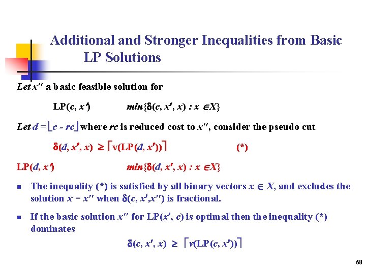
Additional and Stronger Inequalities from Basic LP Solutions Let x″ a basic feasible solution for LP(c, x ) min{d(c, x , x) : x X} Let d = c - rc where rc is reduced cost to x″, consider the pseudo cut d(d, x , x) v(LP(d, x )) LP(d, x ) n n (*) min{d(d, x , x) : x X} The inequality (*) is satisfied by all binary vectors x X, and excludes the solution x = x″ when d(c, x , x″) is fractional. If the basic solution x″ for LP(x , c) is optimal then the inequality (*) dominates d(c, x , x) v(LP(c, x )) 68
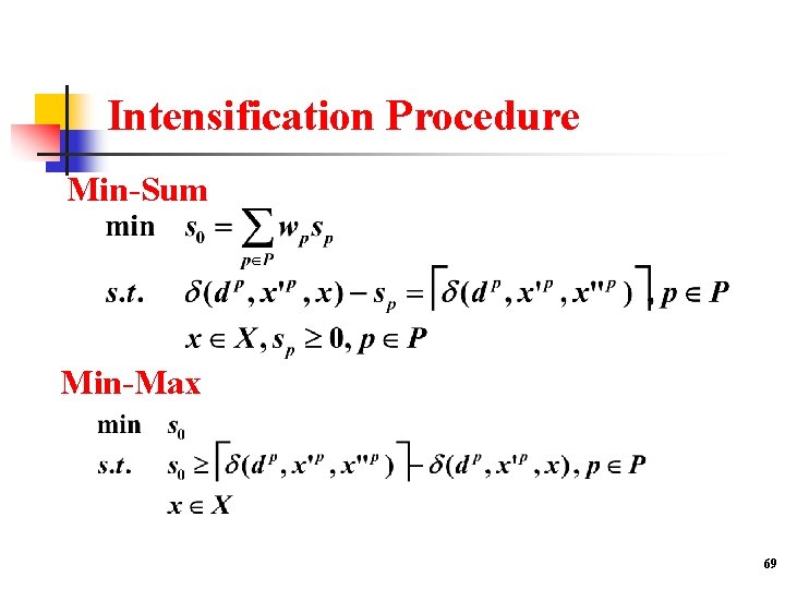
Intensification Procedure Min-Sum Min-Max 69
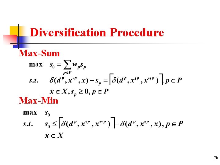
Diversification Procedure Max-Sum Max-Min 70

Conclusions n n n Many MIP problems resist to be solved by the best current B&B and B&C methods. Metaheuristics can likewise profit from generating inequalities to supplement their basic functions. This framework can be exploited in generating target objectives, employing both adaptive memory ideas and newer ones proposed here. 71
Some Prospects n n n Extension to other problems Improve the implementation of dominance rules Integrate intensification and diversification Strengthen the use of memory Parallel versions 72
- Slides: 72