Combinatorial Testing Slides modified from Aditya Marthurs Fo

Combinatorial Testing Slides modified from Aditya Marthur’s Fo. ST chapter 4.

Learning Objectives § What are test configurations? How do they differ from test sets? § Why combinatorial design? § IPO algorithm © Aditya P. Mathur 2009

Test configuration § Software applications are often designed to work in a variety of environments. Combinations of factors such as the operating system, network connection, and hardware platform, lead to a variety of environments. § An environment is characterized by combination of hardware and software. § Each environment corresponds to a given set of values for each factor, known as a test configuration. © Aditya P. Mathur 2009

Test configuration: Example § Windows XP, Dial-up connection, and a PC with 512 MB of main memory, is one possible configuration. § Different versions of operating systems and printer drivers, can be combined to create several test configurations for a printer. § To ensure high reliability across the intended environments, the application must be tested under as many test configurations, or environments, as possible. The number of such test configurations could be exorbitantly large making it impossible to test the application exhaustively. © Aditya P. Mathur 2009

Test configuration and test set § While a test configuration is a combination of factors corresponding to hardware and software within which an application is to operate, a test set is a collection of test cases. Each test case consists of input values and expected output. § Techniques we shall learn are useful in deriving test configurations as well as test sets. © Aditya P. Mathur 2009

Motivation § While testing a program with one or more input variables, each test run of a program often requires at least one value for each variable. § For example, a program to find the greatest common divisor of two integers x and y requires two values, one corresponding to x and the other to y. © Aditya P. Mathur 2009

Motivation [2] While equivalence partitioning discussed earlier offers a set of guidelines to design test cases, it suffers from two shortcomings: (a) It raises the possibility of a large number of sub-domains in the partition. (b) It lacks guidelines on how to select inputs from various subdomains in the partition. © Aditya P. Mathur 2009

Motivation [3] The number of sub-domains in a partition of the input domain increases in direct proportion to the number and type of input variables, and especially so when multidimensional partitioning is used. Once a partition is determined, one selects at random a value from each of the sub-domains. Such a selection procedure, especially when using uni-dimensional equivalence partitioning, does not account for the possibility of faults in the program under test that arise due to specific interactions amongst values of different input variables. © Aditya P. Mathur 2009

Motivation [4] While boundary values analysis leads to the selection of test cases that test a program at the boundaries of the input domain, other interactions in the input domain might remain untested. We will learn several techniques for generating test configurations or test sets that are small even when the set of possible configurations or the input domain and the number of sub-domains in its partition, is large and complex. © Aditya P. Mathur 2009

Modeling: Input and configuration space [1] The input space of a program P consists of k-tuples of values that could be input to P during execution. The configuration space of P consists of all possible settings of the environment variables under which P could be used. Consider program P that takes two integers x>0 and y>0 as inputs. The input space of P is the set of all pairs of positive nonzero integers. © Aditya P. Mathur 2009

Modeling: Input and configuration space [2] Now suppose that this program is intended to be executed under the Windows and the Mac. OS operating system, through the Netscape or Safari browsers, and must be able to print to a local or a networked printer. The configuration space of P consists of triples (X, Y, Z) where X represents an operating system, Y a browser, and Z a local or a networked printer. © Aditya P. Mathur 2009

Factors and levels Consider a program P that takes n inputs corresponding to variables X 1, X 2, . . Xn. We refer to the inputs as factors. The inputs are also referred to as test parameters or as values. Let us assume that each factor may be set at any one from a total of ci, 1 i n values. Each value assignable to a factor is known as a level. |F| refers to the number of levels for factor F. © Aditya P. Mathur 2009

Factor combinations A set of values, one for each factor, is known as a factor combination. For example, suppose that program P has two input variables X and Y. Let us say that during an execution of P, X and Y may each assume a value from the set {a, b, c} and {d, e, f}, respectively. Thus we have 2 factors and 3 levels for each factor. This leads to a total of 32=9 factor combinations, namely (a, d), (a, e), (a, f), (b, d), (b, e), (b, f), (c, d), (c, e), and (c, f). © Aditya P. Mathur 2009

Factor combinations: Too large? In general, for k factors with each factor assuming a value from a set of n values, the total number of factor combinations is nk. Suppose now that each factor combination yields one test case. For many programs, the number of tests generated for exhaustive testing could be exorbitantly large. For example, if a program has 15 factors with 4 levels each, the total number of tests is 415 ~109. Executing a billion tests might be impractical for many software applications. © Aditya P. Mathur 2009

Example: Pizza Delivery Service (PDS) [1] A PDS takes orders online, checks for their validity, and schedules Pizza for delivery. A customer is required to specify the following four items as part of the online order: Pizza size, Toppings list, Delivery address and a home phone number. Let us denote these four factors by S, T, A, and P, respectively. © Aditya P. Mathur 2009

Pizza Delivery Service (PDS): Specs Suppose now that there are three varieties for size: Large, Medium, and Small. There is a list of 6 toppings from which to select. In addition, the customer can customize the toppings. The delivery address consists of customer name, one line of address, city, and the zip code. The phone number is a numeric string possibly containing the dash (``--") separator. © Aditya P. Mathur 2009

PDS: Input space model The total number of factor combinations is 24+23=24. Suppose we consider 6+1=7 levels for Toppings. Number of combinations= 24+5 x 23+23+5 x 22=84. Different types of values for Address and Phone number will further increase the combinations © Aditya P. Mathur 2009

Example: Testing a GUI The Graphical User Interface of application T consists of three menus labeled File, Edit, and Format. We have three factors in T. Each of these three factors can be set to any of four levels. Thus we have a total 43=64 factor combinations. © Aditya P. Mathur 2009

Example: The UNIX sort utility The sort utility has several options and makes an interesting example for the identification of factors and levels. The command line for sort is given below. sort [-cmu] [-ooutput] [-Tdirectory] [-y [ kmem]] [-zrecsz] [dfi. Mnr] [-b] [ tchar] [-kkeydef] [+pos 1[-pos 2]] [file. . . ] We have identified a total of 20 factors for the sort command. The levels listed in Table 11. 1 of the book lead to a total of approximately 1. 9 x 109 combinations. © Aditya P. Mathur 2009

Example: Compatibility testing There is often a need to test a web application on different platforms to ensure that any claim such as ``Application X can be used under Windows and Mac OS X” are valid. Here we consider a combination of hardware, operating system, and a browser as a platform. Let X denote a Web application to be tested for compatibility. Given that we want X to work on a variety of hardware, OS, and browser combinations, it is easy to obtain three factors, i. e. hardware, OS, and browser. © Aditya P. Mathur 2009

Compatibility testing: Factor levels © Aditya P. Mathur 2009

Compatibility testing: Combinations There are 75 factor combinations. However, some of these combinations are infeasible. For example, Mac OS 10. 2 is an OS for the Apple computers and not for the Dell Dimension series PCs. Similarly, the Safari browser is used on Apple computers and not on the PC in the Dell Series. While various editions of the Windows OS can be used on an Apple computer using an OS bridge such as the Virtual PC, we assume that this is not the case for testing application X. © Aditya P. Mathur 2009

Compatibility testing: Reduced combinations The discussion above leads to a total of 40 infeasible factor combinations corresponding to the hardware-OS combination and the hardware-browser combination. Thus in all we are left with 35 platforms on which to test X. Note that there is a large number of hardware configurations under the Dell Dimension Series. These configurations are obtained by selecting from a variety of processor types, e. g. Pentium versus Athelon, processor speeds, memory sizes, and several others. © Aditya P. Mathur 2009

Compatibility testing: Reduced combinations-2 While testing against all configurations will lead to more thorough testing of application X, it will also increase the number of factor combinations, and hence the time to test. © Aditya P. Mathur 2009

Combinatorial test design process Modeling of input space or the environment is not exclusive and one might apply either one or both depending on the application under test. © Aditya P. Mathur 2009

Combinatorial test design process: steps Step 1: Model the input space and/or the configuration space. The model is expressed in terms of factors and their respective levels. Step 2: The model is input to a combinatorial design procedure to generate a combinatorial object which is simply an array of factors and levels. Such an object is also known as a factor covering design. Step 3: The combinatorial object generated is used to design a test set or a test configuration as the requirement might be. Steps 2 and 3 can be automated. © Aditya P. Mathur 2009

Combinatorial test design process: test inputs Each combination obtained from the levels listed in Table 4. 1 can be used to generate many test inputs. For example, consider the combination in which all factors are set to ``Unused" except the -o option which is set to ``Valid File" and the file option that is set to ``Exists. ” Two sample test cases are: t 1: sort -o afile bfile t 2: sort -o cfile dfile Is one of the above tests sufficient? © Aditya P. Mathur 2009

Combinatorial test design process: summary Combination of factor levels is used to generate one or more test cases. For each test case, the sequence in which inputs are to be applied to the program under test must be determined by the tester. Further, the factor combinations do not indicate in any way the sequence in which the generated tests are to be applied to the program under test. This sequence too must be determined by the tester. The sequencing of tests generated by most test generation techniques must be determined by the tester and is not a unique characteristic of test generated in combinatorial testing. © Aditya P. Mathur 2009

Fault model Faults aimed at by the combinatorial design techniques are known as interaction faults. We say that an interaction fault is triggered when a certain combination of t 1 input values causes the program containing the fault to enter an invalid state. Of course, this invalid state must propagate to a point in the program execution where it is observable and hence is said to reveal the fault. © Aditya P. Mathur 2009

t-way interaction faults Faults triggered by some value of an input variable, i. e. t=1, regardless of the values of other input variables, are known as simple faults. For t=2, the faults are known as pairwise interaction faults. In general, for any arbitrary value of t, the faults are known as t-way interaction faults. © Aditya P. Mathur 2009

Pairwise interaction fault: Example Correct output: f(x, y, z)-g(x, y) when X=x 1 and Y=y 1. This is a pairwise interaction fault due to the interaction between factors X and Y. © Aditya P. Mathur 2009

3 -way interaction fault: Example This fault is triggered by all inputs such that x+y x-y and z 0. However, the fault is revealed only by the following two of the eight possible input combinations: x= -1, y=1, z=1 and x=-1, y=-1, z=1. © Aditya P. Mathur 2009

Fault vectors Given a set of k factors f 1, f 2, . . , fk, each at qi, 1 i k levels, a vector V of factor levels is (l 1, l 2, . . , lk), where li, 1 i k is a specific level for the corresponding factor. V is also known as a run. A run V is a fault vector for program P if the execution of P against a test case derived from V triggers a fault in P. V is considered as a t-fault vector if any t k elements in V are needed to trigger a fault in P. Note that a t-way fault vector for P triggers a t-way fault in P. © Aditya P. Mathur 2009

Fault vectors: Example The input domain consists of three factors x, y, and z each having two levels. There is a total of eight runs. For example, (1, 1, 1) and (1, -1, 0) are two runs. Of these eight runs, (-1, 1, 1) and (-1, 1) are three fault vectors that trigger the 3 -way fault. (x 1, y 1, *) is a 2 -way fault vector given that the values x 1 and y 1 trigger the two-way fault. © Aditya P. Mathur 2009

Covering array A covering array CA(N, k, s, t) is an N x k matrix in which entries are from a finite set S of s symbols such that each N x t subarray contains each possible t-tuple at least times. N denotes the number of runs, k the number factors, s, the number of levels for each factor, t the strength, and the index While generating test cases or test configurations for a software application, we use =1. © Aditya P. Mathur 2009

Covering array: Example © Aditya P. Mathur 2009

Mixed level covering arrays A mixed-level covering array is a covering array in which factors have different levels. © Aditya P. Mathur 2009

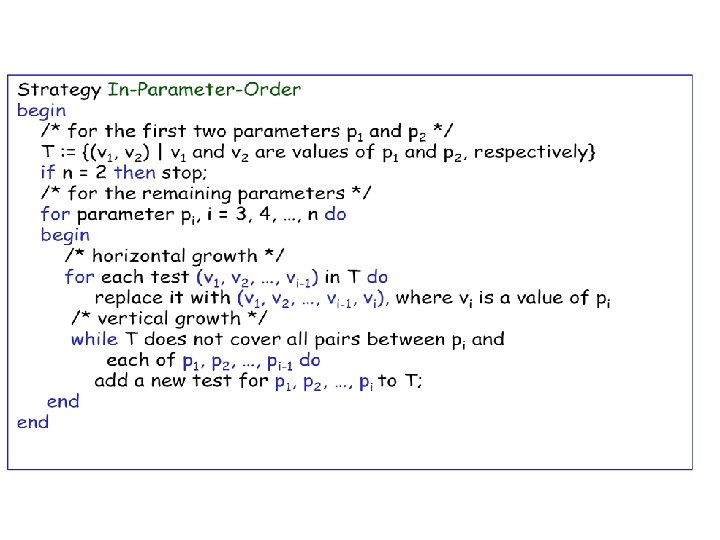
Generating mixed level covering arrays We will now study a procedure due to Lei and Tai for the generation of mixed level covering arrays. The procedure is known as In-parameter Order (IPO) procedure. Inputs: (a) n 2: Number of parameters (factors). (b) Number of values (levels) for each parameter. Output: MCA © Aditya P. Mathur 2009

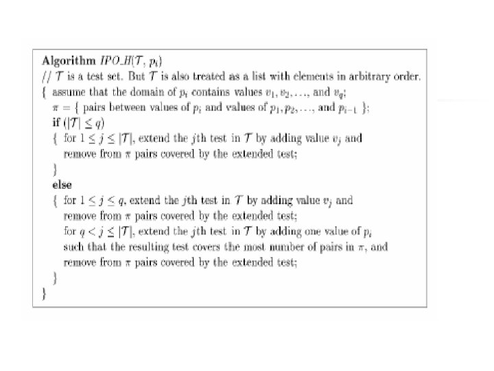
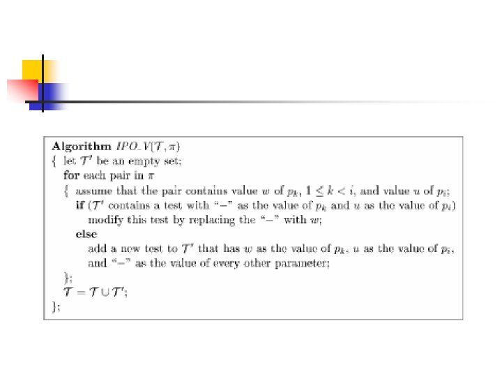
IPO procedure Consists of three steps: Step 1: Main procedure. Step 2: Horizontal growth. Step 3: Vertical growth. © Aditya P. Mathur 2009

IPO procedure: Example Consider a program with three factors A, B, and C. A assumes values from the set {a 1, a 2, a 3}, B from the set {b 1, b 2}, and C from the set {c 1, c 2, c 3}. We want to generate a mixed level covering array for these three factors. . We begin by applying the Main procedure which is the first step in the generation of an MCA using the IPO procedure. © Aditya P. Mathur 2009

IPO procedure: main procedure Main: Step 1: Construct all runs that consist of pairs of values of the first two parameters. We obtain the following set. Let us denote the elements of as t 1, t 2, …t 6. The entire IPO procedure would terminate at this point if the number of parameters n=2. In our case n=3 hence we continue with horizontal growth. © Aditya P. Mathur 2009

IPO procedure: Horizontal growth HG: Step 1: Compute the set of all pairs AP between parameters A and C, and parameters B and C. This leads us to the following set of fifteen pairs. HG: Step 2: AP is the set of pairs yet to be covered. Let T’ denote the set of runs obtained by extending the runs in T. At this point T’ is empty as we have not extended any run in T. © Aditya P. Mathur 2009

Horizontal growth: Extend HG: Steps 3, 4: Expand t 1, t 2, t 3 by appending c 1, c 2, c 3. This gives us: t 1’=(a 1, b 1, c 1), t 2’=(a 1, b 2, c 2), and t 3’=(a 2, b 1, c 3) Update T’ which becomes {a 1, b 1, c 1), (a 1, b 2, c 2), (a 2, b 1, c 3)} Update pairs remaining to be covered AP={(a 1, c 3), (a 2, c 1), (a 2, c 2), (a 3, c 1), (a 3, c 2), (a 3, c 3), (b 1, c 2), (b 2, c 1), (b 2, c 3)} Update T’ which becomes {(a 1, b 1, c 1), (a 1, b 2, c 2), (a 2, b 1, c 3)} © Aditya P. Mathur 2009

Horizontal growth: Optimal extension HG. Step 5: We have not extended t 4, t 5, t 6 as C does not have enough elements. We find the best way to extend these in the next step. HG: Step 6: Expand t 4, t 5, t 6 by suitably selected values of C. If we extend t 4=(a 2, b 2) by c 1 then we cover two of the uncovered pairs from AP, namely, (a 2, c 1) and (b 2, c 1). If we extend it by c 2 then we cover one pair from AP. If we extend it by c 3 then we cover one pairs in AP. Thus we choose to extend t 4 by c 1. © Aditya P. Mathur 2009

Horizontal growth: Update and extend remaining T’={(a 1, b 1, c 1), (a 1, b 2, c 2), (a 2, b 1, c 3), (a 2, b 2, c 1)} AP= {(a 1, c 3), (a 2, c 2), (a 3, c 1), (a 3, c 2), (a 3, c 3), (b 1, c 2), (b 2, c 3)}�� HG: Step 6: Similarly we extend t 5 and t 6 by the best possible values of parameter C. This leads to: t 5’=(a 3, b 1, c 3) and t 6’=(a 3, b 2, c 1) T’={(a 1, b 1, c 1), (a 1, b 2, c 2), (a 2, b 1, c 3), (a 2, b 2, c 1), (a 3, b 1, c 3), (a 3, b 2, c 1)} AP= {(a 1, c 3), (a 2, c 2), (a 3, c 2), (b 1, c 2), (b 2, c 3)}�� © Aditya P. Mathur 2009

Horizontal growth: Done We have completed the horizontal growth step. However, we have five pairs remaining to be covered. These are: AP= {(a 1, c 3), (a 2, c 2), (a 3, c 2), (b 1, c 2), (b 2, c 3)} Also, we have generated six complete runs namely: T’={(a 1, b 1, c 1), (a 1, b 2, c 2), (a 2, b 1, c 3), (a 2, b 2, c 1), (a 3, b 1, c 3), (a 3, b 2, c 1)} We now move to the vertical growth step of the main IPO procedure to cover the remaining pairs. © Aditya P. Mathur 2009

Vertical growth For each missing pair p from AP, we will add a new run to T’ such that p is covered. Let us begin with the pair p= (a 1, c 3). The run t= (a 1, *, c 3) covers pair p. Note that the value of parameter Y does not matter and hence is indicated as a * which denotes a don’t care value. Next , consider p=(a 2, c 2). This is covered by the run (a 2, *, c 2) Next , consider p=(a 3, c 2). This is covered by the run (a 3, *, c 2) © Aditya P. Mathur 2009

Vertical growth (contd. ) Next , consider p=(b 2, c 3). We already have (a 1, *, c 3) and hence we can modify it to get the run (a 1, b 2, c 3). Thus p is covered without any new run added. Finally, consider p=(b 1, c 2). We already have (a 3, *, c 2) and hence we can modify it to get the run (a 3, b 1, c 2). Thus p is covered without any new run added. We replace the don’t care entries by an arbitrary value of the corresponding factor and get: T={(a 1, b 1, c 1), (a 1, b 2, c 2), (a 1, b 1, c 3), (a 2, b 1, c 2), (a 2, b 2, c 1), (a 2, b 2, c 3), (a 3, b 1, c 3), (a 3, b 2, c 1), (a 3, b 1, c 2)} © Aditya P. Mathur 2009

Final covering array © Aditya P. Mathur 2009 Run F 1(X) F 2(Y) F 3(Z) 1 1 2 1 2 2 3 1 2 3 4 2 1 2 5 2 1 3 6 2 2 1 7 3 1 2 8 3 1 3 9 3 2 1

Practicalities That completes our presentation of an algorithm to generate covering arrays. A detailed analysis of the algorithm has been given by Lei and Tai offer several other algorithms for horizontal and vertical growth that are faster than the algorithm mentioned here. © Aditya P. Mathur 2009