Collaboration and data sharing in the Distributed Graduate

Collaboration and data sharing in the Distributed Graduate Seminars Role of NCEAS in the DGS Coordination Collaborative webspace Grad Research Associate Informatics support Outreach support & publicity Time & space for synthesis

Collaboration and data sharing in the Distributed Graduate Seminars Organization of this presentation: • Basic problems and solutions in data sharing & collaboration • Introduction to NCEAS collaborative sites • Overview of NCEAS computing research and support

Collaboration and data sharing Collaboration & data stewardship Personal data management problems are magnified in collaboration • Data organization • Data documentation • Data analysis • Data & analysis preservation

“Data Entropy” Michener et al. 1997, Ecological Monographs Time of publication Information content Specific details General details Retirement or career change Accident Death Time

Collaboration and data sharing A personal example. . .

Collaboration and data sharing 2 tables

Collaboration and data sharing Random notes What is this?

Collaboration and data sharing Wash Cres Lake Dec 15 Dont_Use. xls

What if we want to merge files?

Collaboration and data sharing What is this?

Collaboration and data sharing Personal data management problems are magnified in collaboration • Data organization – standardize • Data documentation – standardize descriptions of data (metadata) • Data analysis - document • Data & analysis preservation - protect

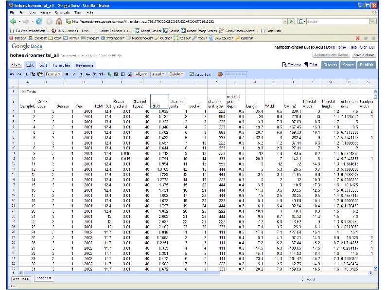
Example – using R for data exploration, analysis and presentation ### Simple Linear Regression - 0+ age Trout in Hoh River, WA against Temp Celsius ### Load data Hoh. Trout<-read. csv("Hoh_Trout 0_Temp. csv") ### See full metadata in Rosenberger, E. E. , S. L. Katz, J. Mc. Millan, G. Pess. , and S. E. Hampton. In prep. Hoh River trout habitat associations. ### http: //knb. ecoinformatics. org/knb/style/skins/nceas/ ### Look at the data Hoh. Trout plot(TROUT ~ TEMPC, data=Hoh. Trout) ### Log Transform the independent variable (x+1) - this method for transform creates a new column in the data frame Hoh. Trout$LNtrout<-log(Hoh. Trout$TROUT+1) ### Plot the log-transformed y against x ### First I'll ask R to open new windows for subsequent graphs with the windows command windows() plot(LNtrout ~ TEMPC, data=Hoh. Trout) ### Regression of log trout abundance on log temperature mod. r <- lm(LNtrout ~ TEMPC, data=Hoh. Trout) ### add a regression line to the plot. abline(mod. r) ### Check out the residuals in a new plot layout(matrix(1: 4, nr=2)) windows() plot(mod. r, which=1) ### Check out statistics for the regression summary. lm(mod. r)

Example – using R for data exploration, analysis and presentation ### Simple Linear Regression - 0+ age Trout in Hoh River, WA against Temp Celsius ### Load data Hoh. Trout<-read. csv("Hoh_Trout 0_Temp. csv") ### See full metadata in Rosenberger, E. E. , S. L. Katz, J. Mc. Millan, G. Pess. , and S. E. Hampton. In prep. Hoh River trout habitat associations. ### http: //knb. ecoinformatics. org/knb/style/skins/nceas/ ### Look at the data Hoh. Trout plot(TROUT ~ TEMPC, data=Hoh. Trout) ### Log Transform the independent variable (x+1) - this method for transform creates a new column in the data frame Hoh. Trout$LNtrout<-log(Hoh. Trout$TROUT+1) ### Plot the log-transformed y against x ### First I'll ask R to open new windows for subsequent graphs with the windows command windows() plot(LNtrout ~ TEMPC, data=Hoh. Trout) ### Regression of log trout abundance on log temperature mod. r <- lm(LNtrout ~ TEMPC, data=Hoh. Trout) ### add a regression line to the plot. abline(mod. r) ### Check out the residuals in a new plot layout(matrix(1: 4, nr=2)) windows() plot(mod. r, which=1) ### Check out statistics for the regression summary. lm(mod. r) Call: lm(formula = LNtrout ~ TEMPC, data = Hoh. Trout) Residuals: Min 1 Q Median 3 Q Max -1. 7534 -1. 1924 -0. 3294 0. 9304 4. 2231 Coefficients: Estimate Std. Error t value Pr(>|t|) (Intercept) -0. 07545 0. 18220 -0. 414 0. 679 TEMPC 0. 11220 0. 01448 7. 746 1. 74 e-14 *** --Signif. codes: 0 ‘***’ 0. 001 ‘**’ 0. 01 ‘*’ 0. 05 ‘. ’ 0. 1 ‘ ’ 1 Residual standard error: 1. 365 on 1501 degrees of freedom Multiple R-Squared: 0. 03844, Adjusted R-squared: 0. 0378 F-statistic: 60 on 1 and 1501 DF, p-value: 1. 735 e-14

Compare this method to: ### Simple Linear Regression - 0+ age Trout in Hoh River, WA against Temp Celsius ### Load data Hoh. Trout<-read. csv("Hoh_Trout 0_Temp. csv") Copy and paste from Excel ### See full metadata in Rosenberger, E. E. , S. L. Katz, J. Mc. Millan, G. Pess. , and S. E. Hampton. In prep. Hoh River trout habitat associations. ### http: //knb. ecoinformatics. org/knb/style/skins/nceas/ ### Look at the data Hoh. Trout plot(TROUT ~ TEMPC, data=Hoh. Trout) Graph in Sigma. Plot ### Log Transform the independent variable (x+1) - this method for transform creates a new column in the data frame Hoh. Trout$LNtrout<-log(Hoh. Trout$TROUT+1) Log-transform in Excel ### Plot the log-transformed y against x ### First I'll ask R to open new windows for subsequent graphs with the windows command Copy and paste new file windows() plot(LNtrout ~ TEMPC, data=Hoh. Trout) Graph in Sigma. Plot ### Regression of log trout abundance on log temperature mod. r <- lm(LNtrout ~ TEMPC, data=Hoh. Trout) Analyze in Systat ### add a regression line to the plot. abline(mod. r) ### Check out the residuals in a new plot layout(matrix(1: 4, nr=2)) windows() plot(mod. r, which=1) ### Check out statistics for the regression summary. lm(mod. r) Graph in Sigma. Plot

Collaboration & data stewardship • Personal data management problems are magnified in collaboration • Data organization – standardize • Data documentation – standardize metadata • Data analysis - document • Data & analysis preservation - protect

Collaboration and data sharing Personal data management problems are magnified in collaboration • Data organization – standardize • Data documentation – standardize metadata • Data analysis - document • Data & analysis preservation - protect

“Data Entropy” Michener et al. 1997, Ecological Monographs Time of publication Information content Specific details General details Retirement or career change Accident Death Time

Technological solutions • Databases that protect original data structure (e. g. , not “sorting” in Excel) • Statistical software that documents transformations, sorts, analysis, etc. (e. g. , R, Matlab, SAS, JMP, PRIMER) • Free software for data management & analysis • Morpho, free software that standardizes descriptions of data (metadata) • Central collaborative space organizing communications

Communication for collaboration Emphasis is on accessibility Open to collaborators Archived for the future Highly organized Searchable

Communication for collaboration n o i s Emphasis is on accessibility s u sc m i D oru F s g o Bl t a h C ail Em Open to collaborators √ √ √ Archived for the future √ √ Highly organized √ Searchable √ √

NCEAS Collaborative Websites What we have in place: User-editable website Discussion Forums Realtime chat with archived transcripts What others have used: Skype Google Docs Zoho Go. To. Meeting

NCEAS Collaborative Websites Easy file uploading PDF library Discussion boards Wiki-style collaborative page editing Real-time chat

NCEAS Collaborative Websites Easy file uploading PDF library Discussion boards Wiki-style collaborative page editing Real-time chat All is searchable Click to go to the DGS Website

NCEAS Collaborative Websites Making useful tools for the students and faculty is critical Technology helps, but many of the problems are more social than technical Find a mixture that helps you get your work done

traits-dgs. nceas. ucsb. edu Please create an account: http: //traits-dgs. nceas. ucsb. edu/ Explore a previous site: http: //dgs. nceas. ucsb. edu name: student password: stu 00

General NCEAS Tech Support

NCEAS recycles!

NCEAS Tech Support

NCEAS collaboration support http: //help. nceas. ucsb. edu

NCEAS Tech Support

NCEAS Analytical Support

NCEAS Tech Support

Ecoinformatics at NCEAS

Metadata - Describing your data Metadata – description of your data – makes data useful Needed to Assess & interpret data Provide context for data

Metadata - Describing your data Metadata – description of your data – makes data useful Needed to Assess & interpret data Provide context for data But how to handle different styles of describing data? e. g. , abundance vs. biomass

Metadata - Describing your data Metadata – description of your data – makes data useful Needed to Assess & interpret data Provide context for data But how to handle different styles of describing data? e. g. , abundance vs. biomass Ecological Metadata Language (EML) Metadata standard Human-readable, yet machine-interpretable

Metadata - Describing your data What EML metadata looks like. . .

Metadata - Describing your data 1. Use our basic web interface 2. Install Morpho desktop software (free) Create & save metadata using wizards a. Manage data on your own computer b. Share metadata/data with the broader community c. Share with specific colleagues: set access privileges Search and locate data and metadata on the network

Metadata - Describing your data

Search knb. ecoinformatics. org NCEAS – LTER Network – OBFS – PISCO – ESA – UC Natural Reserve System – and more

NCEAS recycles!