Cointegrating VAR Models and Probability Forecasting Applied to

Cointegrating VAR Models and Probability Forecasting: Applied to a Small Open Economy Gustavo Sánchez April 2009

Summary n VEC and Cointegrating VAR Models n n Estimate Parameters Probability Forecasting Simulate Forecasts n Summary Statistics to estimate probabilities of events n

Point Forecast and Confidence Interval

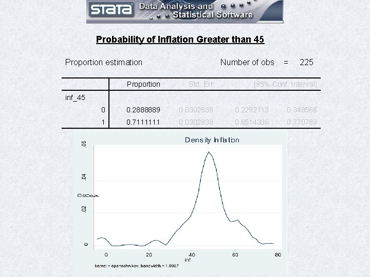
Probability of Inflation Greater than 45 Proportion estimation Number of obs = 225 Proportion Std. Err. [95% Conf. Interval] 0 0. 2888889 0. 0302838 0. 2292113 0. 348566 1 0. 7111111 0. 0302838 0. 6514336 0. 770789 inf_45

Cointegrating VAR models n n Based on the vector error correction (VEC) model specification. The specification assumes that the economic theory characterizes the long-run equilibrium behavior The short-run fluctuations represent deviations from that equilibrium. The short-run and long-run (economic) concepts are linked to the statistical concept of stationarity.

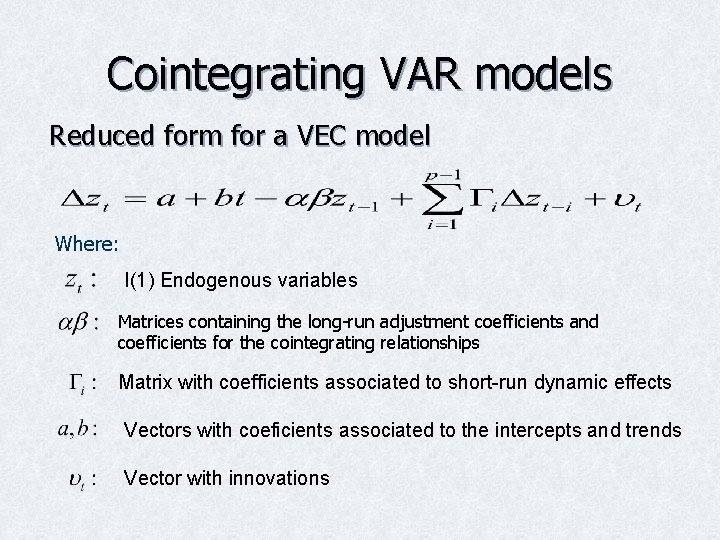
Cointegrating VAR models Reduced form for a VEC model Where: I(1) Endogenous variables Matrices containing the long-run adjustment coefficients and coefficients for the cointegrating relationships Matrix with coefficients associated to short-run dynamic effects Vectors with coeficients associated to the intercepts and trends Vector with innovations

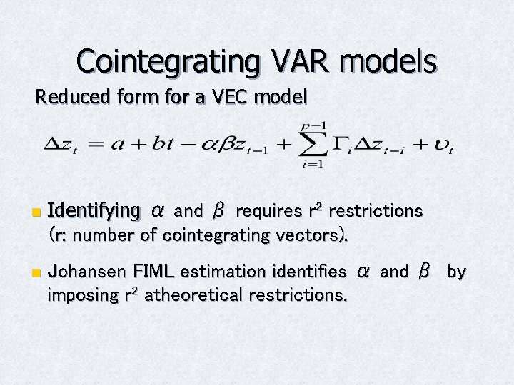
Cointegrating VAR models Reduced form for a VEC model n n Identifying α and β requires r 2 restrictions (r: number of cointegrating vectors). Johansen FIML estimation identifies α and β by imposing r 2 atheoretical restrictions.

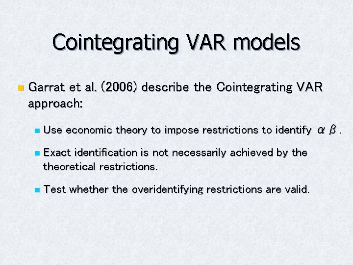
Cointegrating VAR models n Garrat et al. (2006) describe the Cointegrating VAR approach: n Use economic theory to impose restrictions to identify αβ. n Exact identification is not necessarily achieved by theoretical restrictions. n Test whether the overidentifying restrictions are valid.

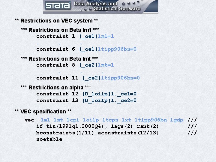
** Restrictions on VEC system ** *** Restrictions on Beta lm 1 *** constraint 1 [_ce 1]lm 1=1. . . constraint 6 [_ce 1]ltipp 906 bn=0 *** Restrictions on Beta lmt *** constraint 8 [_ce 2]lmt=1. . . constraint 11 [_ce 2]ltipp 906 bn=0 *** Restrictions on alpha *** constraint 12 [D_loilp]l. _ce 1=0 constraint 13 [D_loilp]l. _ce 2=0 ** VEC specification ** vec lm 1 lmt lcpi loilp ltcpn lxt ltipp 906 bn lgdp /// if tin(1991 q 1, 2008 Q 4), lags(2) rank(2) /// bconstraints(1/11) aconstraints(12/13) /// noetable

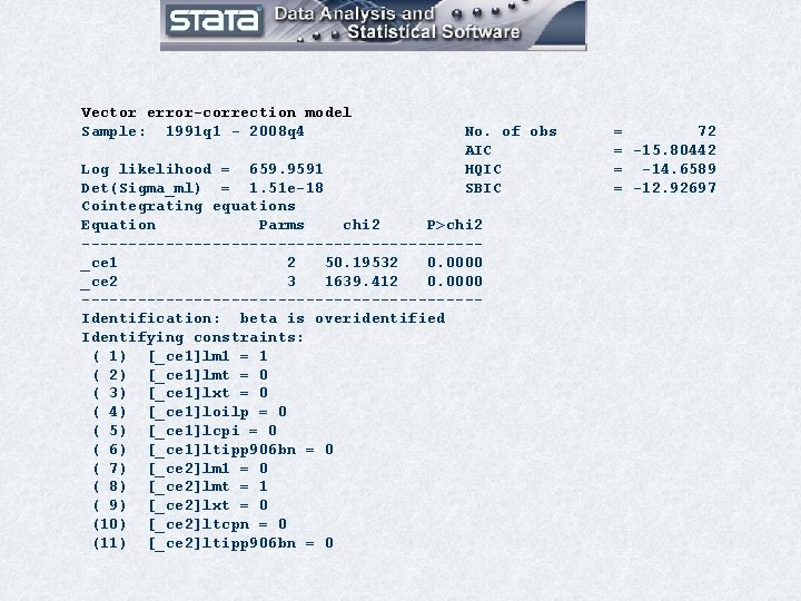
Vector error-correction model Sample: 1991 q 1 - 2008 q 4 No. of obs AIC HQIC SBIC Log likelihood = 659. 9591 Det(Sigma_ml) = 1. 51 e-18 Cointegrating equations Equation Parms chi 2 P>chi 2 ---------------------_ce 1 2 50. 19532 0. 0000 _ce 2 3 1639. 412 0. 0000 ---------------------Identification: beta is overidentified Identifying constraints: ( 1) [_ce 1]lm 1 = 1 ( 2) [_ce 1]lmt = 0 ( 3) [_ce 1]lxt = 0 ( 4) [_ce 1]loilp = 0 ( 5) [_ce 1]lcpi = 0 ( 6) [_ce 1]ltipp 906 bn = 0 ( 7) [_ce 2]lm 1 = 0 ( 8) [_ce 2]lmt = 1 ( 9) [_ce 2]lxt = 0 (10) [_ce 2]ltcpn = 0 (11) [_ce 2]ltipp 906 bn = 0 = 72 = -15. 80442 = -14. 6589 = -12. 92697

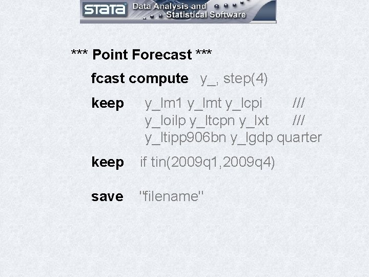
*** Point Forecast *** fcast compute y_, step(4) keep y_lm 1 y_lmt y_lcpi /// y_loilp y_ltcpn y_lxt /// y_ltipp 906 bn y_lgdp quarter keep if tin(2009 q 1, 2009 q 4) save "filename"

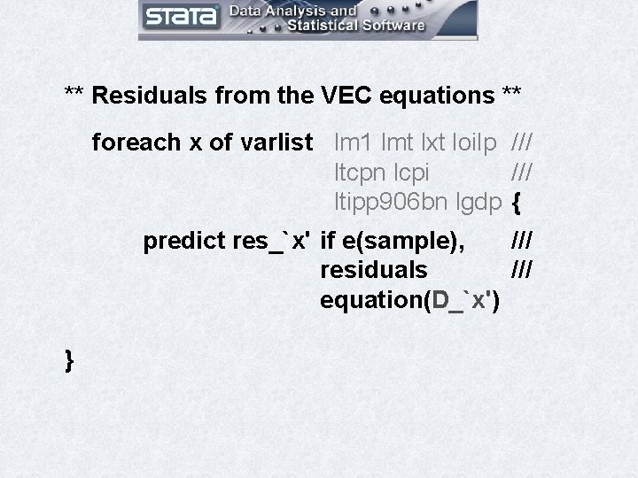
** Residuals from the VEC equations ** foreach x of varlist lm 1 lmt lxt loilp /// ltcpn lcpi /// ltipp 906 bn lgdp { predict res_`x' if e(sample), /// residuals /// equation(D_`x') }

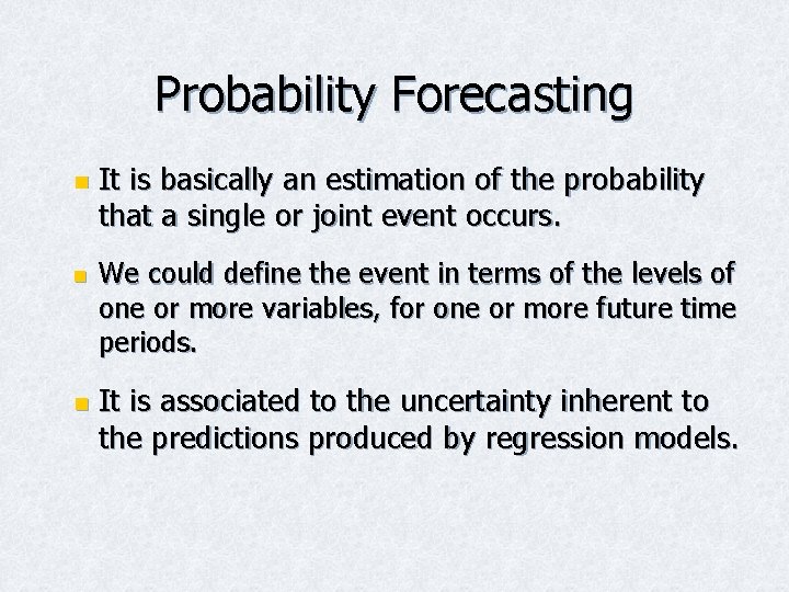
Probability Forecasting n n n It is basically an estimation of the probability that a single or joint event occurs. We could define the event in terms of the levels of one or more variables, for one or more future time periods. It is associated to the uncertainty inherent to the predictions produced by regression models.

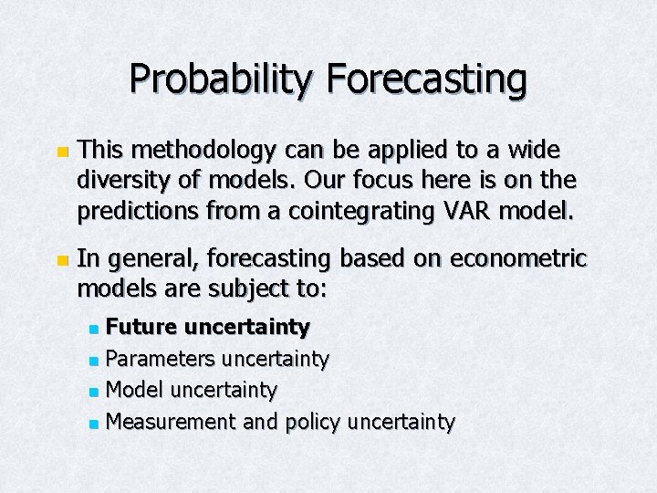
Probability Forecasting n n This methodology can be applied to a wide diversity of models. Our focus here is on the predictions from a cointegrating VAR model. In general, forecasting based on econometric models are subject to: Future uncertainty n Parameters uncertainty n Model uncertainty n Measurement and policy uncertainty n

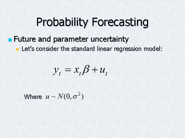
Probability Forecasting n Future and parameter uncertainty n Let’s consider the standard linear regression model: Where

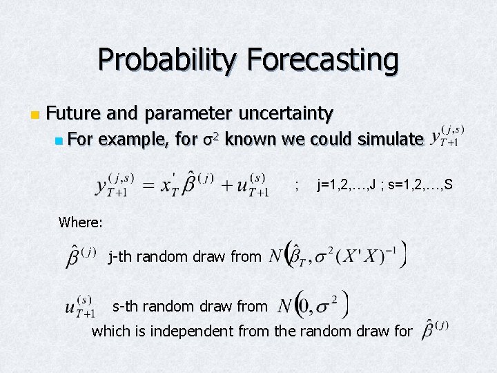
Probability Forecasting n Future and parameter uncertainty n For example, for σ2 known we could simulate ; j=1, 2, …, J ; s=1, 2, …, S Where: j-th random draw from s-th random draw from which is independent from the random draw for

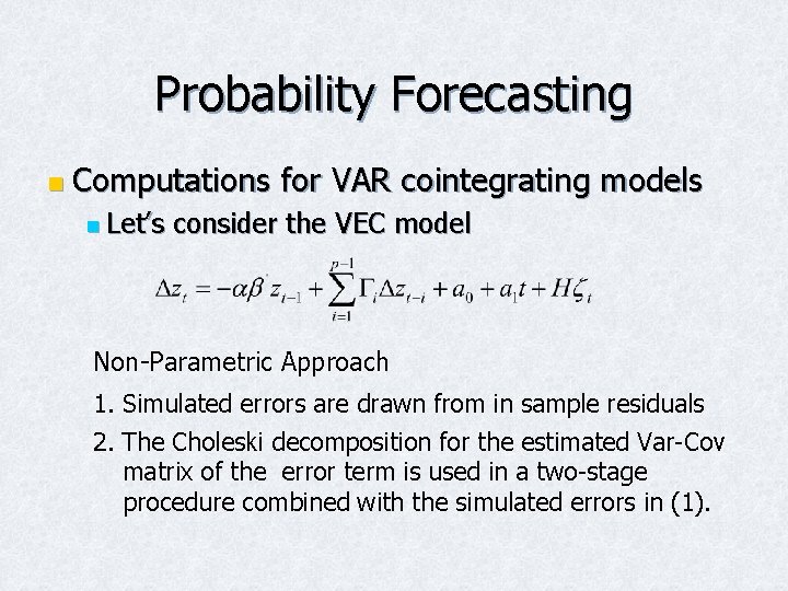
Probability Forecasting n Computations for VAR cointegrating models n Let’s consider the VEC model Non-Parametric Approach 1. Simulated errors are drawn from in sample residuals 2. The Choleski decomposition for the estimated Var-Cov matrix of the error term is used in a two-stage procedure combined with the simulated errors in (1).

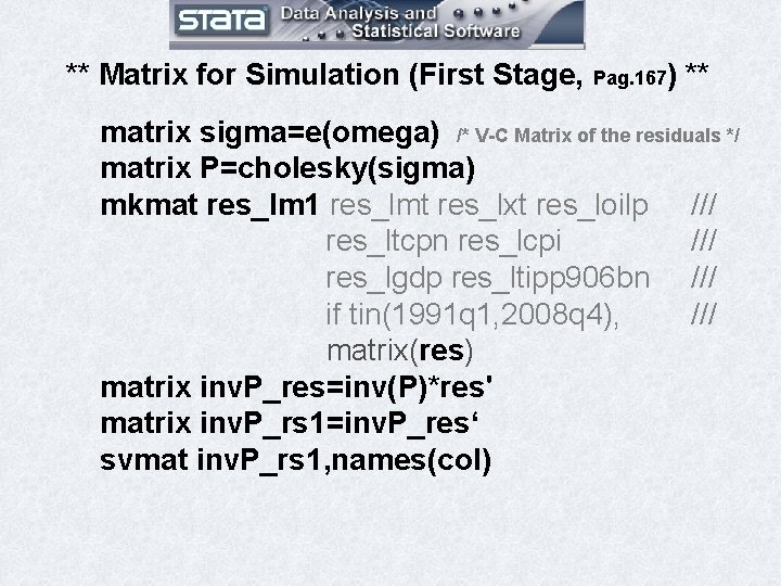
** Matrix for Simulation (First Stage, Pag. 167) ** matrix sigma=e(omega) /* V-C Matrix of the residuals */ matrix P=cholesky(sigma) mkmat res_lm 1 res_lmt res_lxt res_loilp /// res_ltcpn res_lcpi /// res_lgdp res_ltipp 906 bn /// if tin(1991 q 1, 2008 q 4), /// matrix(res) matrix inv. P_res=inv(P)*res' matrix inv. P_rs 1=inv. P_res‘ svmat inv. P_rs 1, names(col)

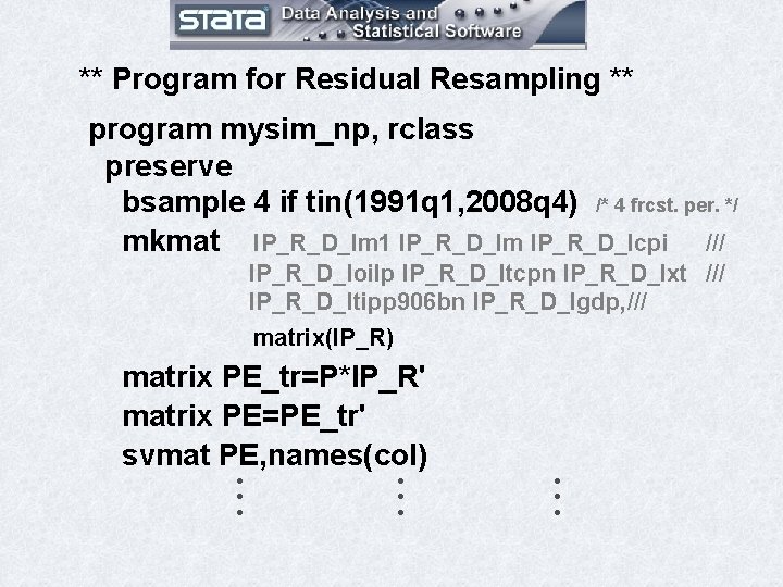
** Program for Residual Resampling ** program mysim_np, rclass preserve bsample 4 if tin(1991 q 1, 2008 q 4) /* 4 frcst. per. */ mkmat IP_R_D_lm 1 IP_R_D_lm IP_R_D_lcpi /// IP_R_D_loilp IP_R_D_ltcpn IP_R_D_lxt /// IP_R_D_ltipp 906 bn IP_R_D_lgdp, /// matrix(IP_R) matrix PE_tr=P*IP_R' matrix PE=PE_tr' svmat PE, names(col) ● ● ● ● ●

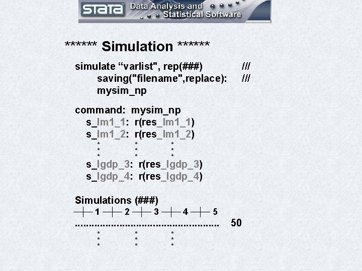
****** Simulation ****** simulate “varlist", rep(###) saving("filename", replace): mysim_np /// command: mysim_np s_lm 1_1: r(res_lm 1_1) s_lm 1_2: r(res_lm 1_2) ● ● ● ● ● s_lgdp_3: r(res_lgdp_3) s_lgdp_4: r(res_lgdp_4) Simulations (###) ─┼─ 1 ─┼─ 2 ─┼─ 3 ─┼─ 4 ─┼─ 5 . . . ● ● ● ● ● 50

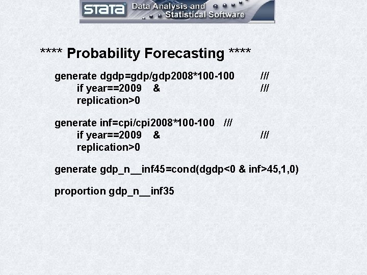
**** Probability Forecasting **** generate dgdp=gdp/gdp 2008*100 -100 if year==2009 & replication>0 generate inf=cpi/cpi 2008*100 -100 /// if year==2009 & replication>0 /// /// generate gdp_n__inf 45=cond(dgdp<0 & inf>45, 1, 0) proportion gdp_n__inf 35

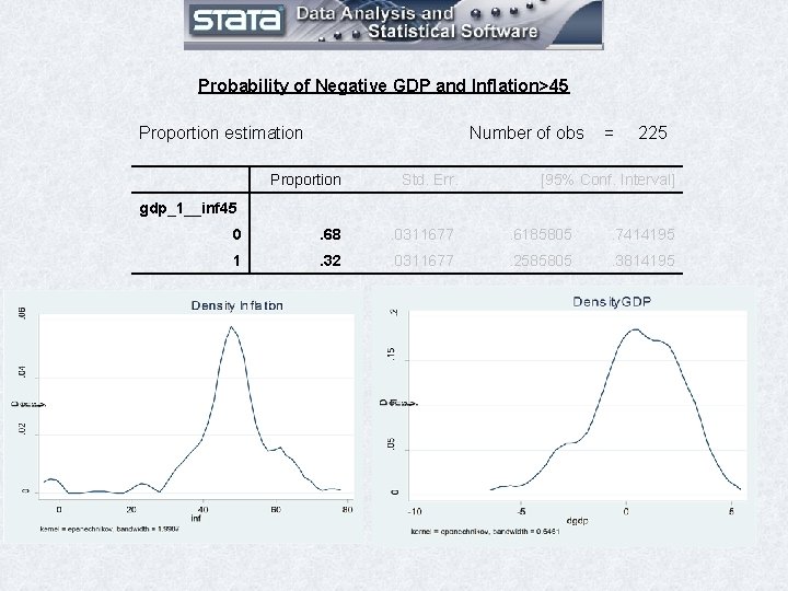
Probability of Negative GDP and Inflation>45 Proportion estimation Number of obs = 225 Proportion Std. Err. [95% Conf. Interval] 0 . 68 . 0311677 . 6185805 . 7414195 1 . 32 . 0311677 . 2585805 . 3814195 gdp_1__inf 45

Cointegrating VAR Models and Probability Forecasting: Applied to a Small Open Economy Gustavo Sánchez April 2009