Cognitive Computer Vision Kingsley Sage khs 20sussex ac

Cognitive Computer Vision Kingsley Sage khs 20@sussex. ac. uk and Hilary Buxton hilaryb@sussex. ac. uk Prepared under ECVision Specific Action 8 -3 http: //www. ecvision. org

Lecture 7 l (Hidden) Markov Models – – What are they? What can you do with them?

So why are HMMs relevant to Cognitive CV? l l Provides a well-founded methodology for reasoning about temporal events One method that you can use as a basis for our model of expectation

Markov Models l Markov Models are used to represent and model temporal relationships, e. g. : Ø Ø Motion of objects in a tracker Gestures Interpreting sign language Speech recognition

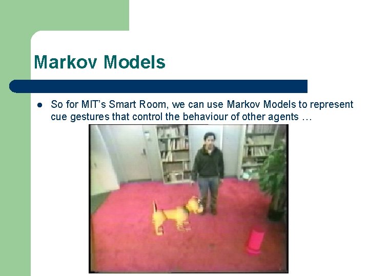
Markov Models l So for MIT’s Smart Room, we can use Markov Models to represent cue gestures that control the behaviour of other agents …

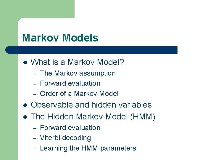
Markov Models l What is a Markov Model? – – – l l The Markov assumption Forward evaluation Order of a Markov Model Observable and hidden variables The Hidden Markov Model (HMM) – – – Forward evaluation Viterbi decoding Learning the HMM parameters

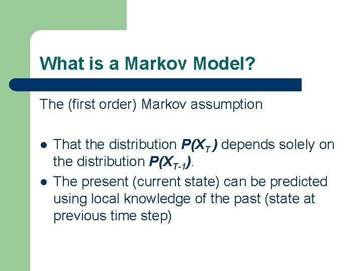
What is a Markov Model? The (first order) Markov assumption l l That the distribution P(XT ) depends solely on the distribution P(XT-1). The present (current state) can be predicted using local knowledge of the past (state at previous time step)

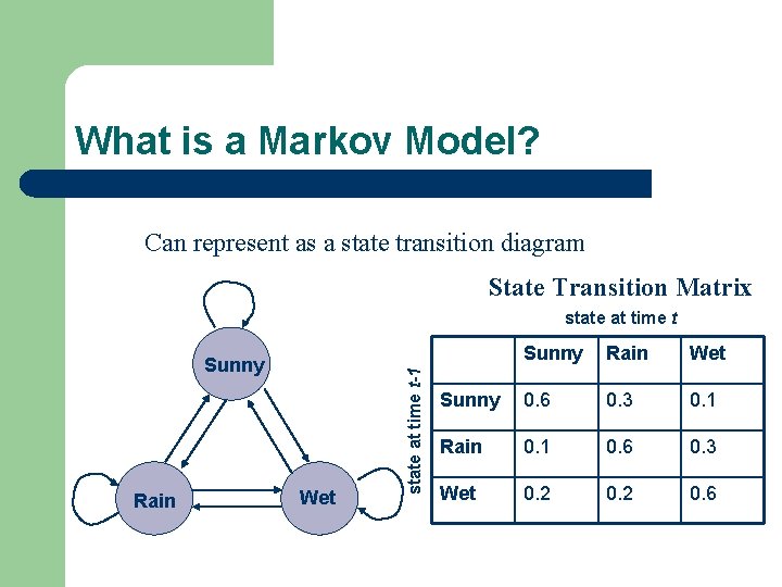
What is a Markov Model? Can represent as a state transition diagram State Transition Matrix Sunny Rain Wet state at time t-1 state at time t Sunny Rain Wet Sunny 0. 6 0. 3 0. 1 Rain 0. 1 0. 6 0. 3 Wet 0. 2 0. 6

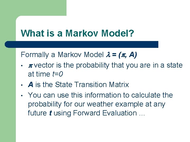
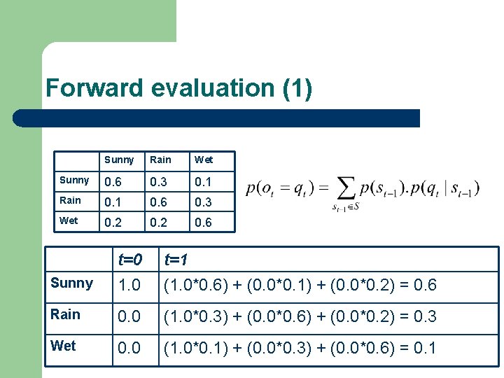
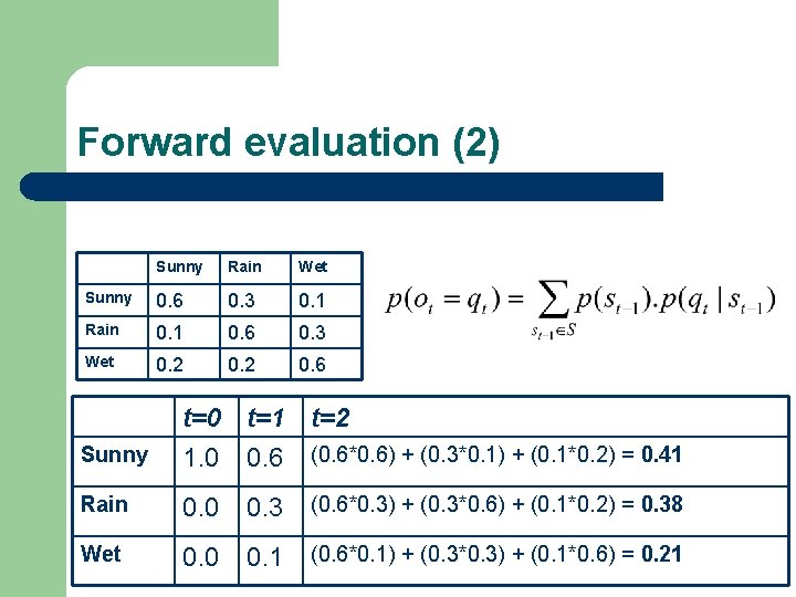
What is a Markov Model? Formally a Markov Model = ( , A) • vector is the probability that you are in a state at time t=0 • A is the State Transition Matrix • You can use this information to calculate the probability for our weather example at any future t using Forward Evaluation …

Forward evaluation (1) Sunny Rain Wet Sunny 0. 6 0. 3 0. 1 Rain 0. 1 0. 6 0. 3 Wet 0. 2 0. 6 Sunny t=0 1. 0 t=1 (1. 0*0. 6) + (0. 0*0. 1) + (0. 0*0. 2) = 0. 6 Rain 0. 0 (1. 0*0. 3) + (0. 0*0. 6) + (0. 0*0. 2) = 0. 3 Wet 0. 0 (1. 0*0. 1) + (0. 0*0. 3) + (0. 0*0. 6) = 0. 1

Forward evaluation (2) Sunny Rain Wet Sunny 0. 6 0. 3 0. 1 Rain 0. 1 0. 6 0. 3 Wet 0. 2 0. 6 Sunny t=0 t=1 t=2 1. 0 0. 6 (0. 6*0. 6) + (0. 3*0. 1) + (0. 1*0. 2) = 0. 41 Rain 0. 0 0. 3 (0. 6*0. 3) + (0. 3*0. 6) + (0. 1*0. 2) = 0. 38 Wet 0. 0 0. 1 (0. 6*0. 1) + (0. 3*0. 3) + (0. 1*0. 6) = 0. 21

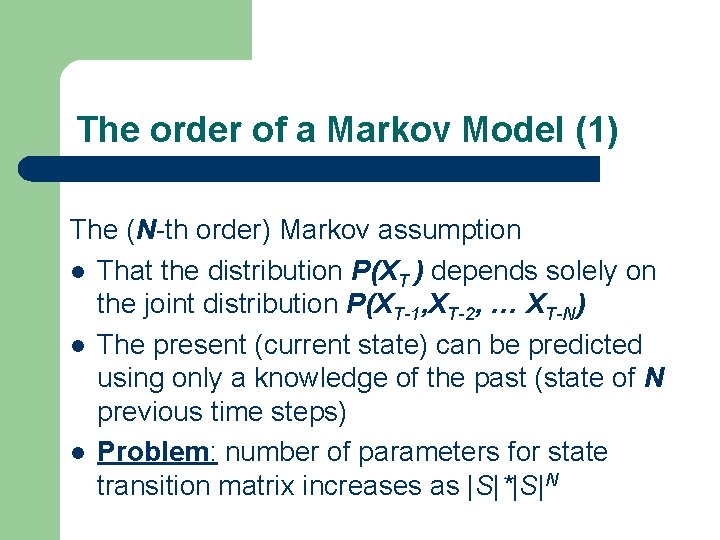
The order of a Markov Model (1) The (N-th order) Markov assumption l That the distribution P(XT ) depends solely on the joint distribution P(XT-1, XT-2, … XT-N) l The present (current state) can be predicted using only a knowledge of the past (state of N previous time steps) l Problem: number of parameters for state transition matrix increases as |S|*|S|N

Before we can discuss Hidden Markov Models (HMMs) … l Observable and hidden variables: – – l A variable is observable if its value can be directly measured, or given as an Observation sequence O A variable is hidden if its value cannot be measured directly, but we can infer its value indirectly So …

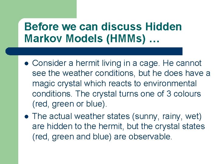
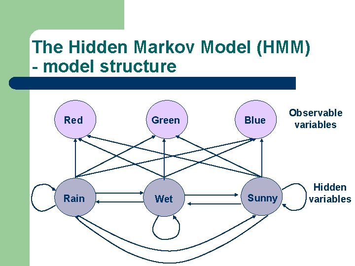
Before we can discuss Hidden Markov Models (HMMs) … l l Consider a hermit living in a cage. He cannot see the weather conditions, but he does have a magic crystal which reacts to environmental conditions. The crystal turns one of 3 colours (red, green or blue). The actual weather states (sunny, rainy, wet) are hidden to the hermit, but the crystal states (red, green and blue) are observable.

The Hidden Markov Model (HMM) - model structure Red Rain Green Wet Blue Sunny Observable variables Hidden variables

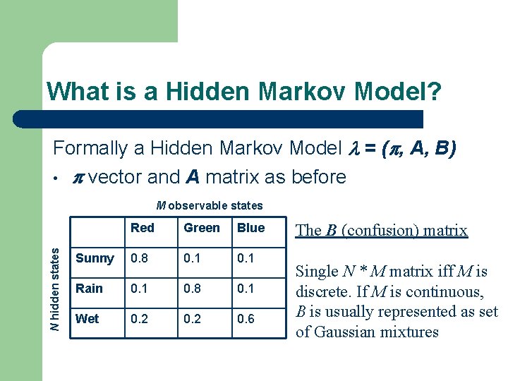
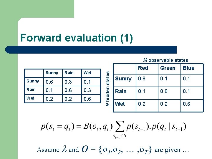
What is a Hidden Markov Model? Formally a Hidden Markov Model = ( , A, B) • vector and A matrix as before N hidden states M observable states Red Green Blue Sunny 0. 8 0. 1 Rain 0. 1 0. 8 0. 1 Wet 0. 2 0. 6 The B (confusion) matrix Single N * M matrix iff M is discrete. If M is continuous, B is usually represented as set of Gaussian mixtures

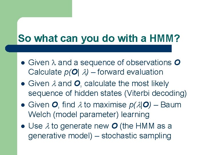
So what can you do with a HMM? l l Given and a sequence of observations O Calculate p(O| ) – forward evaluation Given and O, calculate the most likely sequence of hidden states (Viterbi decoding) Given O, find to maximise p( |O) – Baum Welch (model parameter) learning Use to generate new O (the HMM as a generative model) – stochastic sampling

Forward evaluation (1) Sunny Rain Wet Sunny 0. 6 0. 3 0. 1 Rain 0. 1 0. 6 0. 3 Wet 0. 2 0. 6 Assume and N hidden states M observable states Red Green Blue Sunny 0. 8 0. 1 Rain 0. 1 0. 8 0. 1 Wet 0. 2 0. 6 O = {o 1, o 2, … , o. T} are given …

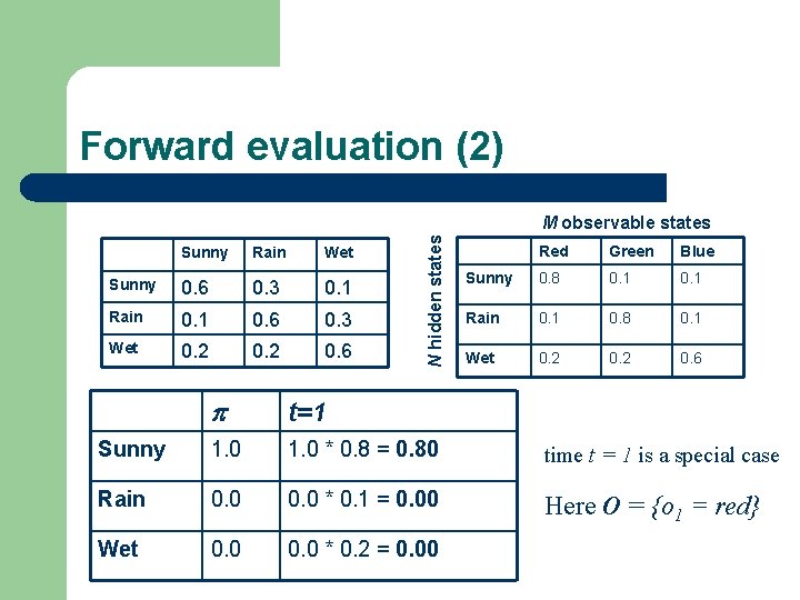
Forward evaluation (2) Sunny Rain Wet Sunny 0. 6 0. 3 0. 1 Rain 0. 1 0. 6 0. 3 Wet 0. 2 0. 6 N hidden states M observable states Red Green Blue Sunny 0. 8 0. 1 Rain 0. 1 0. 8 0. 1 Wet 0. 2 0. 6 t=1 Sunny 1. 0 * 0. 8 = 0. 80 time t = 1 is a special case Rain 0. 0 * 0. 1 = 0. 00 Here O = {o 1 = red} Wet 0. 0 * 0. 2 = 0. 00

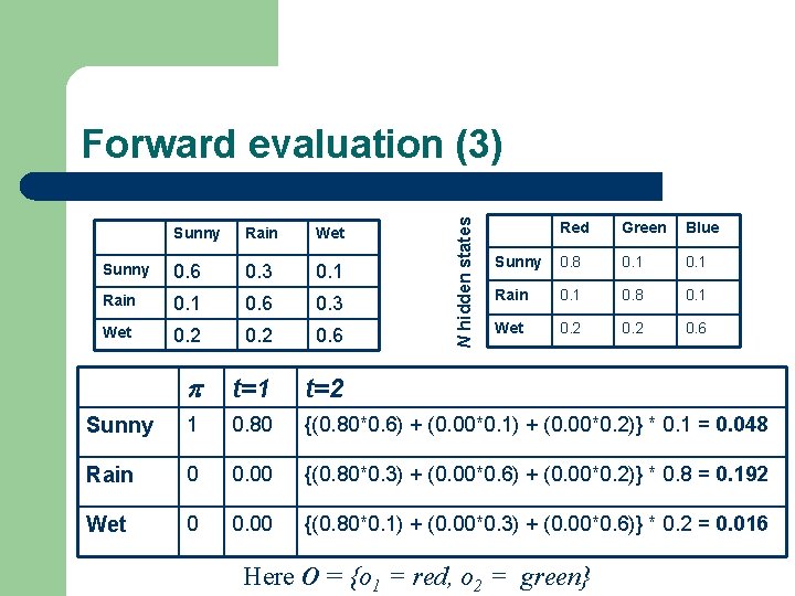
N hidden states Forward evaluation (3) Red Green Blue Sunny 0. 8 0. 1 Rain 0. 1 0. 8 0. 1 Wet 0. 2 0. 6 Sunny Rain Wet Sunny 0. 6 0. 3 0. 1 Rain 0. 1 0. 6 0. 3 Wet 0. 2 0. 6 t=1 t=2 Sunny 1 0. 80 {(0. 80*0. 6) + (0. 00*0. 1) + (0. 00*0. 2)} * 0. 1 = 0. 048 Rain 0 0. 00 {(0. 80*0. 3) + (0. 00*0. 6) + (0. 00*0. 2)} * 0. 8 = 0. 192 Wet 0 0. 00 {(0. 80*0. 1) + (0. 00*0. 3) + (0. 00*0. 6)} * 0. 2 = 0. 016 Here O = {o 1 = red, o 2 = green}

Seminar l l l Prior assumption Practical issues in computing the forward evaluation matrix Measure of likelihood per observation symbol Backwards evaluation Reference: “An Introduction to Hidden Markov Models”, L. R. Rabiner & B. H. Juang, IEEE ASSP Magazine, January 1986

Further reading l l l Try reading the Rabiner paper (it’s quite friendly really) … Mixture of Gaussians: many maths books will cover MOG. Non-trivial maths involved … Variable length Markov Models: “The Power of Amnesia”, D. Ron, Y. Singer and N. Tishby, In Advances in Neural Information Processing Systems (NIPS), vol 6, pp 176 -183, 1994

Summary l l l An N-th order Markov model incorporates the assumption that the future depends only on the last N timesteps In Markov model reasoning over time, we use a state transition matrix A and a vector representing the probabilities at time step t=1 We use a matrix B which maps the observation O to the hidden states

Next time … l Gaussian mixtures and HMMs with continuous valued data