Cognitive Computer Vision 3 R 400 Kingsley Sage

Cognitive Computer Vision 3 R 400 Kingsley Sage Room 5 C 16, Pevensey III khs 20@sussex. ac. uk

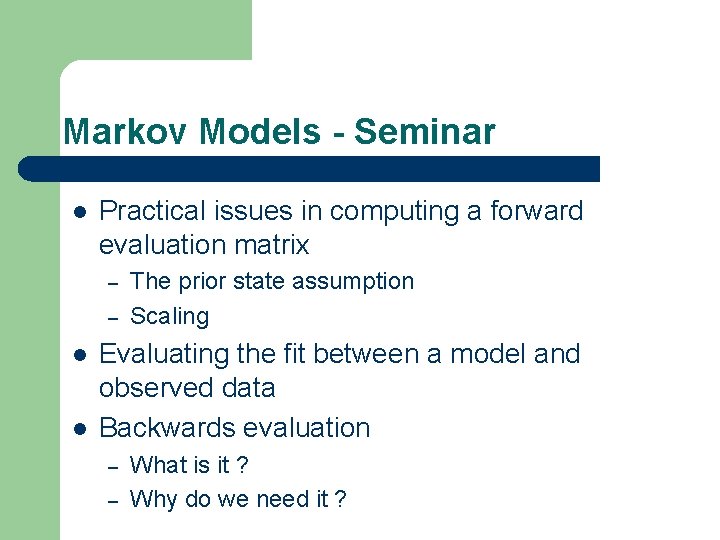
Markov Models - Seminar l Practical issues in computing a forward evaluation matrix – – l l The prior state assumption Scaling Evaluating the fit between a model and observed data Backwards evaluation – – What is it ? Why do we need it ?

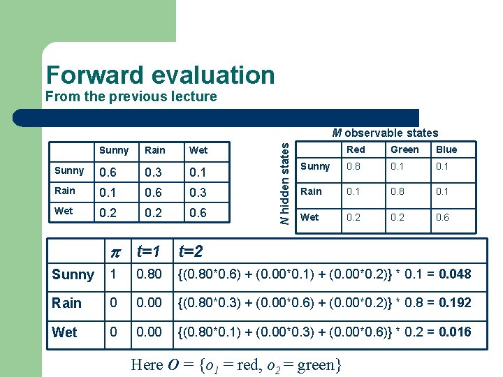
Forward evaluation From the previous lecture Sunny Rain Wet Sunny 0. 6 0. 3 0. 1 Rain 0. 1 0. 6 0. 3 Wet 0. 2 0. 6 N hidden states M observable states Red Green Blue Sunny 0. 8 0. 1 Rain 0. 1 0. 8 0. 1 Wet 0. 2 0. 6 t=1 t=2 Sunny 1 0. 80 {(0. 80*0. 6) + (0. 00*0. 1) + (0. 00*0. 2)} * 0. 1 = 0. 048 Rain 0 0. 00 {(0. 80*0. 3) + (0. 00*0. 6) + (0. 00*0. 2)} * 0. 8 = 0. 192 Wet 0 0. 00 {(0. 80*0. 1) + (0. 00*0. 3) + (0. 00*0. 6)} * 0. 2 = 0. 016 Here O = {o 1 = red, o 2 = green}

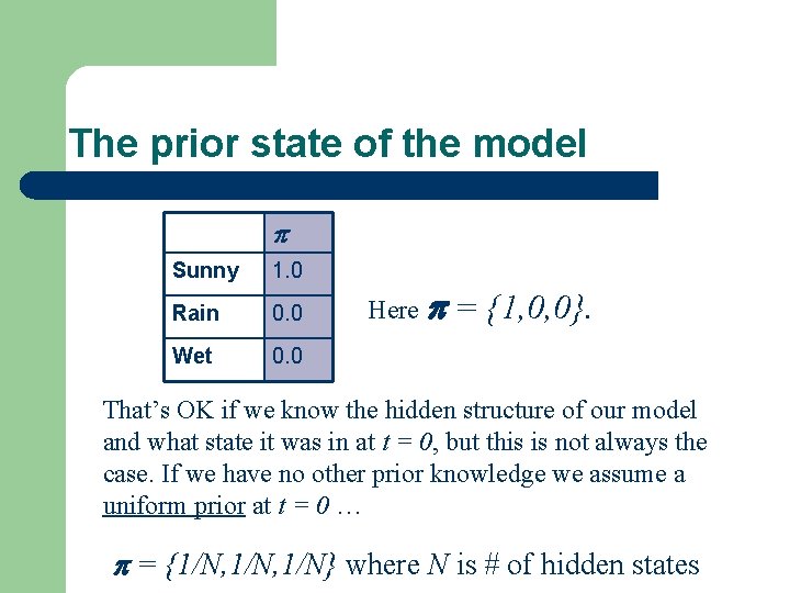
The prior state of the model Sunny 1. 0 Rain 0. 0 Wet 0. 0 Here = {1, 0, 0}. That’s OK if we know the hidden structure of our model and what state it was in at t = 0, but this is not always the case. If we have no other prior knowledge we assume a uniform prior at t = 0 … = {1/N, 1/N} where N is # of hidden states

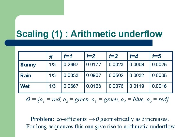
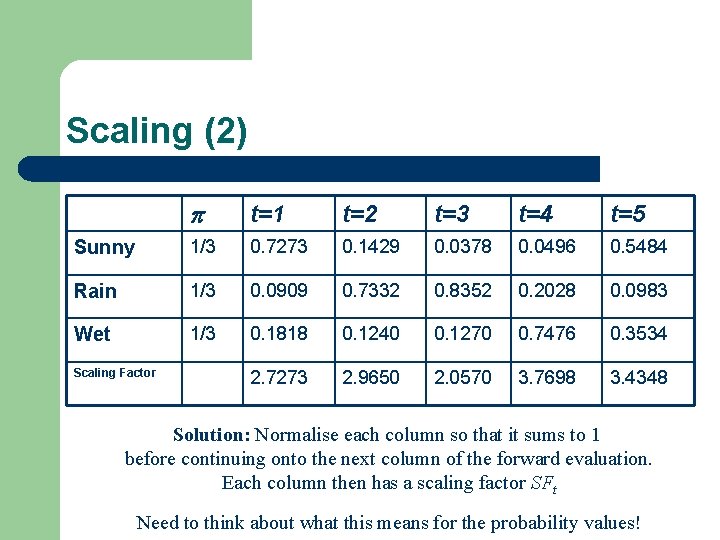
Scaling (1) : Arithmetic underflow t=1 t=2 t=3 t=4 t=5 Sunny 1/3 0. 2667 0. 0177 0. 0023 0. 0008 0. 0025 Rain 1/3 0. 0333 0. 0907 0. 0502 0. 0032 0. 0005 Wet 1/3 0. 0667 0. 0153 0. 0076 0. 0119 0. 0016 O = {o 1 = red, o 2 = green, o 3 = green, o 4 = blue, o 5 = red} Problem: co-efficients 0 geometrically as t increases. For long sequences this can give rise to arithmetic underflow

Scaling (2) t=1 t=2 t=3 t=4 t=5 Sunny 1/3 0. 7273 0. 1429 0. 0378 0. 0496 0. 5484 Rain 1/3 0. 0909 0. 7332 0. 8352 0. 2028 0. 0983 Wet 1/3 0. 1818 0. 1240 0. 1270 0. 7476 0. 3534 2. 7273 2. 9650 2. 0570 3. 7698 3. 4348 Scaling Factor Solution: Normalise each column so that it sums to 1 before continuing onto the next column of the forward evaluation. Each column then has a scaling factor SFt Need to think about what this means for the probability values!

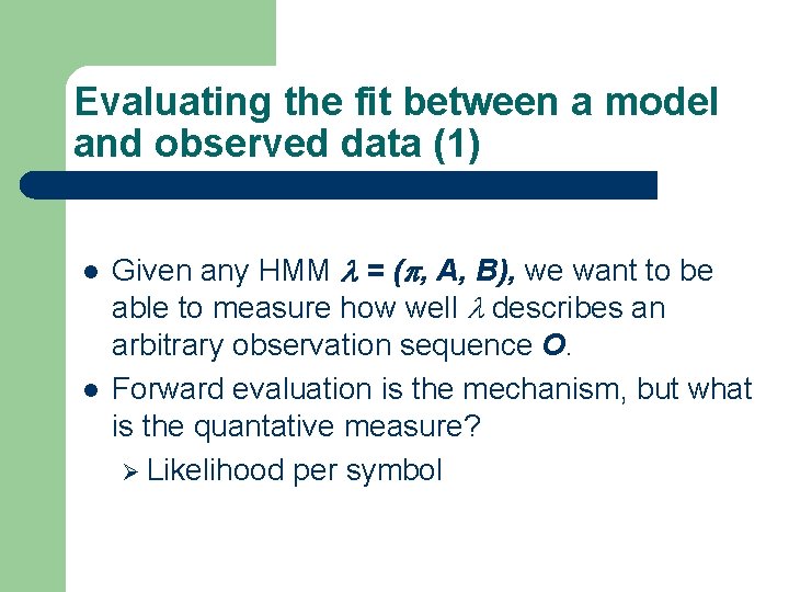
Evaluating the fit between a model and observed data (1) l l Given any HMM = ( , A, B), we want to be able to measure how well describes an arbitrary observation sequence O. Forward evaluation is the mechanism, but what is the quantative measure? Ø Likelihood per symbol

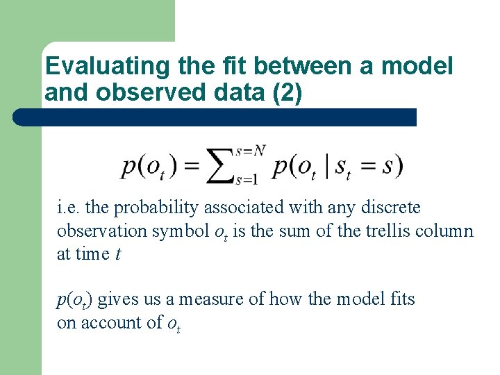
Evaluating the fit between a model and observed data (2) i. e. the probability associated with any discrete observation symbol ot is the sum of the trellis column at time t p(ot) gives us a measure of how the model fits on account of ot

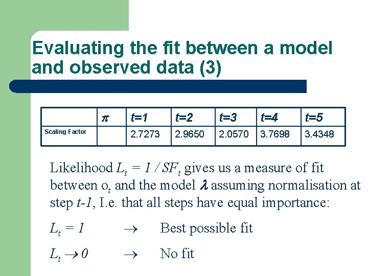
Evaluating the fit between a model and observed data (3) Scaling Factor t=1 t=2 t=3 t=4 t=5 2. 7273 2. 9650 2. 0570 3. 7698 3. 4348 Likelihood Lt = 1 / SFt gives us a measure of fit between ot and the model assuming normalisation at step t-1, I. e. that all steps have equal importance: Lt = 1 Best possible fit Lt 0 No fit

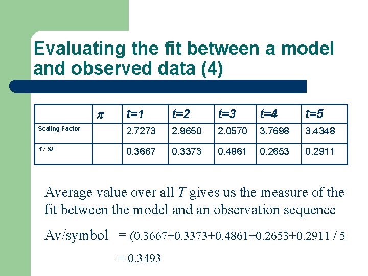
Evaluating the fit between a model and observed data (4) t=1 t=2 t=3 t=4 t=5 Scaling Factor 2. 7273 2. 9650 2. 0570 3. 7698 3. 4348 1 / SF 0. 3667 0. 3373 0. 4861 0. 2653 0. 2911 Average value over all T gives us the measure of the fit between the model and an observation sequence Av/symbol = (0. 3667+0. 3373+0. 4861+0. 2653+0. 2911 / 5 = 0. 3493

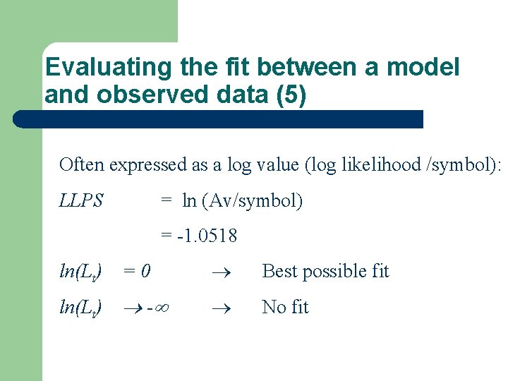
Evaluating the fit between a model and observed data (5) Often expressed as a log value (log likelihood /symbol): LLPS = ln (Av/symbol) = -1. 0518 ln(Lt) = 0 ln(Lt) - Best possible fit No fit

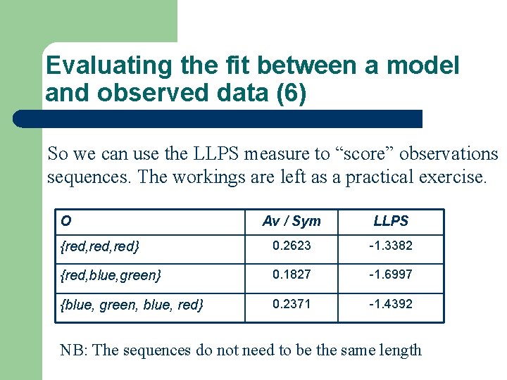
Evaluating the fit between a model and observed data (6) So we can use the LLPS measure to “score” observations sequences. The workings are left as a practical exercise. O Av / Sym LLPS {red, red} 0. 2623 -1. 3382 {red, blue, green} 0. 1827 -1. 6997 {blue, green, blue, red} 0. 2371 -1. 4392 NB: The sequences do not need to be the same length

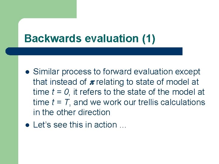
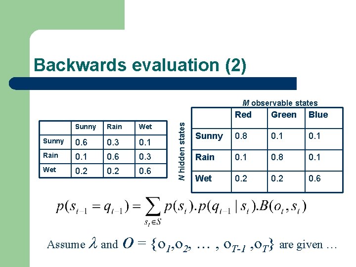
Backwards evaluation (1) l l Similar process to forward evaluation except that instead of relating to state of model at time t = 0, it refers to the state of the model at time t = T, and we work our trellis calculations in the other direction Let’s see this in action …

Backwards evaluation (2) Sunny Rain Wet Sunny 0. 6 0. 3 0. 1 Rain 0. 1 0. 6 0. 3 Wet 0. 2 0. 6 Assume and N hidden states M observable states Red Green Blue Sunny 0. 8 0. 1 Rain 0. 1 0. 8 0. 1 Wet 0. 2 0. 6 O = {o 1, o 2, … , o. T-1 , o. T} are given …

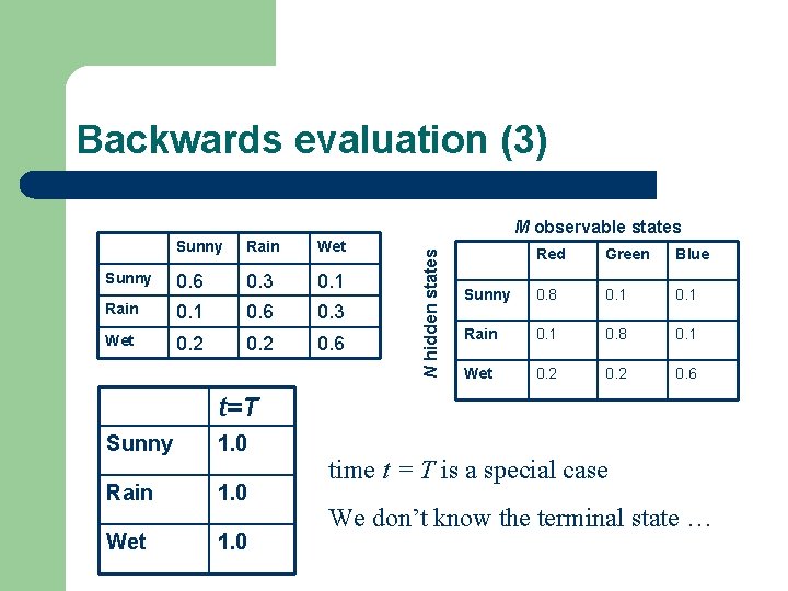
Backwards evaluation (3) Sunny Rain Wet Sunny 0. 6 0. 3 0. 1 Rain 0. 1 0. 6 0. 3 Wet 0. 2 0. 6 N hidden states M observable states Red Green Blue Sunny 0. 8 0. 1 Rain 0. 1 0. 8 0. 1 Wet 0. 2 0. 6 t=T Sunny 1. 0 Rain 1. 0 Wet 1. 0 time t = T is a special case We don’t know the terminal state …

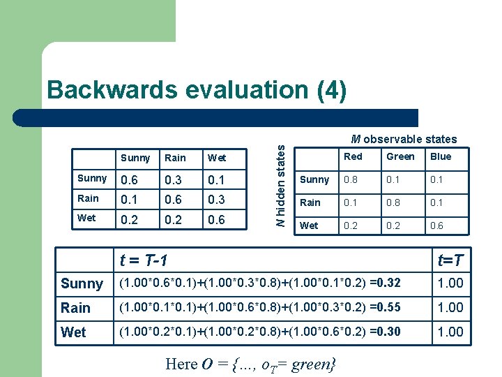
Sunny Rain Wet Sunny 0. 6 0. 3 0. 1 Rain 0. 1 0. 6 0. 3 Wet 0. 2 0. 6 N hidden states Backwards evaluation (4) M observable states Red Green Blue Sunny 0. 8 0. 1 Rain 0. 1 0. 8 0. 1 Wet 0. 2 0. 6 t = T-1 t=T Sunny (1. 00*0. 6*0. 1)+(1. 00*0. 3*0. 8)+(1. 00*0. 1*0. 2) =0. 32 1. 00 Rain (1. 00*0. 1)+(1. 00*0. 6*0. 8)+(1. 00*0. 3*0. 2) =0. 55 1. 00 Wet (1. 00*0. 2*0. 1)+(1. 00*0. 2*0. 8)+(1. 00*0. 6*0. 2) =0. 30 1. 00 Here O = {…, o. T= green}

Backwards evaluation (5) l l l Can calculate p(O| ) just like forward evaluation Same scaling tricks apply Why do we need it then? – – Combine with forward evaluation to create a technique for learning model parameters The forward-backwards algorithm / Baum Welch learning (next lecture)

Coursework Investigating forwards and backwards evaluation and measures of model fit l Need to write code or perform manual calculations, carry out specified experiments and write up a short report l Due <due date> l