CMU SCS Carnegie Mellon Univ Dept of Computer

CMU SCS Carnegie Mellon Univ. Dept. of Computer Science 15 -415/615 - DB Applications C. Faloutsos – A. Pavlo Lecture#14: Implementation of Relational Operations

CMU SCS Administrivia • HW 4 is due this Thursday. • Reminder: Mid-term on Tues March 4 th – Will cover everything up to and including this week’s lectures. – Closed book, one sheet of notes (double-sided) – We will release last year’s exam. Faloutsos/Pavlo CMU SCS 15 -415/615 2

CMU SCS Extended Office Hours • Christos: – Wednesday Feb 26 th 12: 00 pm-1: 00 pm – Friday Feb 28 th 3: 00 pm-5: 00 pm • Andy: – Monday Mar 3 rd 12: 00 pm-2: 00 pm – Or by appointment Faloutsos/Pavlo CMU SCS 15 -415/615 3

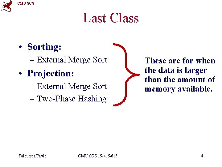
CMU SCS Last Class • Sorting: – External Merge Sort • Projection: – External Merge Sort – Two-Phase Hashing Faloutsos/Pavlo CMU SCS 15 -415/615 These are for when the data is larger than the amount of memory available. 4

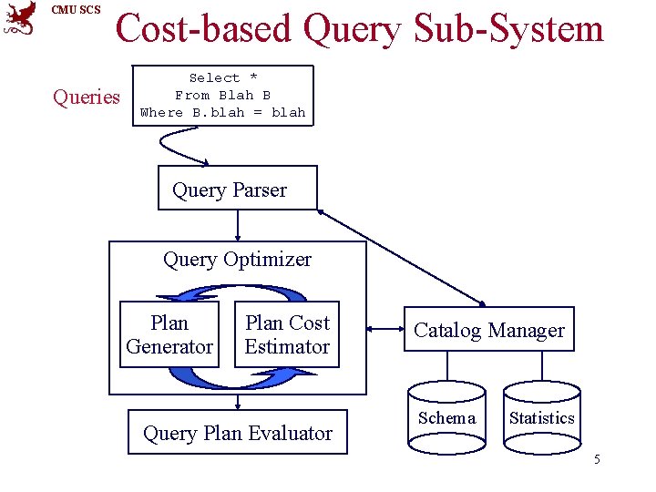
CMU SCS Cost-based Query Sub-System Queries Select * From Blah B Where B. blah = blah Query Parser Query Optimizer Plan Generator Plan Cost Estimator Query Plan Evaluator Catalog Manager Schema Statistics 5

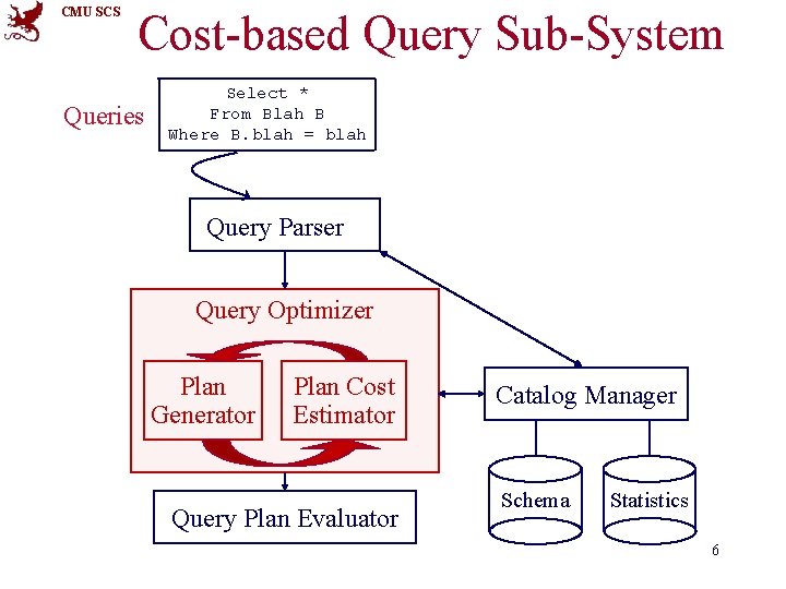
CMU SCS Cost-based Query Sub-System Queries Select * From Blah B Where B. blah = blah Query Parser Query Optimizer Plan Generator Plan Cost Estimator Query Plan Evaluator Catalog Manager Schema Statistics 6

CMU SCS Query Processing • Some database operations are expensive. • The DBMS can greatly improve performance by being “smart” – e. g. , can speed up 1, 000 x over naïve approach Faloutsos/Pavlo CMU SCS 15 -415/615 7

CMU SCS Query Processing • There are clever implementation techniques for operators. • We can exploit “equivalencies” of relational operators to do less work. • Use statistics and cost models to choose among these. Work smarter, not harder. Faloutsos/Pavlo CMU SCS 15 -415/615 8

CMU SCS Today’s Class • Introduction • Selection • Joins Faloutsos/Pavlo CMU SCS 15 -415/615 9

CMU SCS Lame Query Execution • For each SELECT-FROM-WHERE query block – Do cartesian products first – Then do selections + extras: • GROUP BY; HAVING • Projections • ORDER BY • Incredibly inefficient – Huge intermediate results! – Makes small children cry. Faloutsos/Pavlo CMU SCS 15 -415/615 10

CMU SCS Query Optimizer • “Optimizer” is a bit of a misnomer… • Goal is to pick a “good” (i. e. , low expected cost) plan. – Involves choosing access methods, physical operators, operator orders, … – Notion of cost is based on an abstract “cost model” Faloutsos/Pavlo CMU SCS 15 -415/615 11

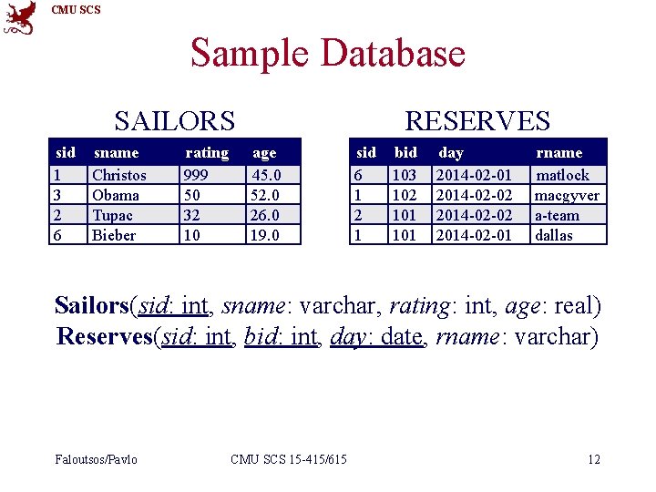
CMU SCS Sample Database SAILORS sid 1 3 2 6 sname Christos Obama Tupac Bieber rating 999 50 32 10 RESERVES age 45. 0 52. 0 26. 0 19. 0 sid 6 1 2 1 bid 103 102 101 day 2014 -02 -01 2014 -02 -02 2014 -02 -01 rname matlock macgyver a-team dallas Sailors(sid: int, sname: varchar, rating: int, age: real) Reserves(sid: int, bid: int, day: date, rname: varchar) Faloutsos/Pavlo CMU SCS 15 -415/615 12

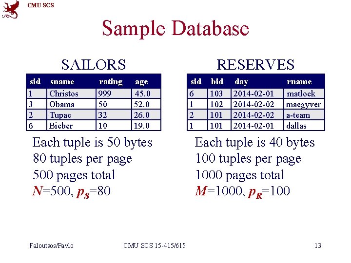
CMU SCS Sample Database SAILORS sid 1 3 2 6 sname Christos Obama Tupac Bieber rating 999 50 32 10 RESERVES age 45. 0 52. 0 26. 0 19. 0 Each tuple is 50 bytes 80 tuples per page 500 pages total N=500, p. S=80 Faloutsos/Pavlo CMU SCS 15 -415/615 sid 6 1 2 1 bid 103 102 101 day 2014 -02 -01 2014 -02 -02 2014 -02 -01 rname matlock macgyver a-team dallas Each tuple is 40 bytes 100 tuples per page 1000 pages total M=1000, p. R=100 13

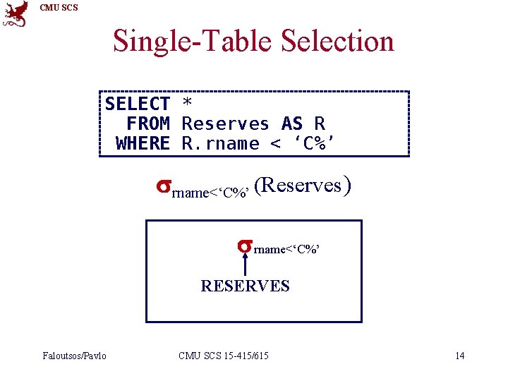
CMU SCS Single-Table Selection SELECT * FROM Reserves AS R WHERE R. rname < ‘C%’ srname<‘C%’ (Reserves) s rname<‘C%’ RESERVES Faloutsos/Pavlo CMU SCS 15 -415/615 14

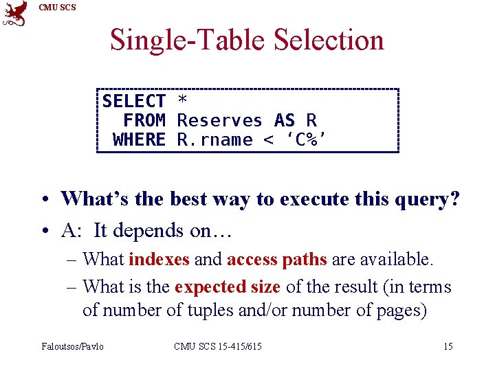
CMU SCS Single-Table Selection SELECT * FROM Reserves AS R WHERE R. rname < ‘C%’ • What’s the best way to execute this query? • A: It depends on… – What indexes and access paths are available. – What is the expected size of the result (in terms of number of tuples and/or number of pages) Faloutsos/Pavlo CMU SCS 15 -415/615 15

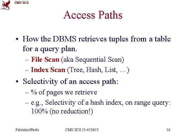
CMU SCS Access Paths • How the DBMS retrieves tuples from a table for a query plan. – File Scan (aka Sequential Scan) – Index Scan (Tree, Hash, List, …) • Selectivity of an access path: – % of pages we retrieve – e. g. , Selectivity of a hash index, on range query: 100% (no reduction!) Faloutsos/Pavlo CMU SCS 15 -415/615 16

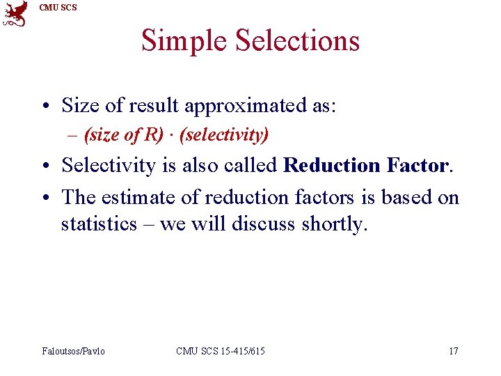
CMU SCS Simple Selections • Size of result approximated as: – (size of R) ∙ (selectivity) • Selectivity is also called Reduction Factor. • The estimate of reduction factors is based on statistics – we will discuss shortly. Faloutsos/Pavlo CMU SCS 15 -415/615 17

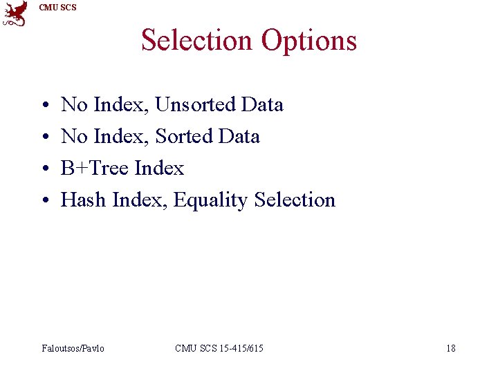
CMU SCS Selection Options • • No Index, Unsorted Data No Index, Sorted Data B+Tree Index Hash Index, Equality Selection Faloutsos/Pavlo CMU SCS 15 -415/615 18

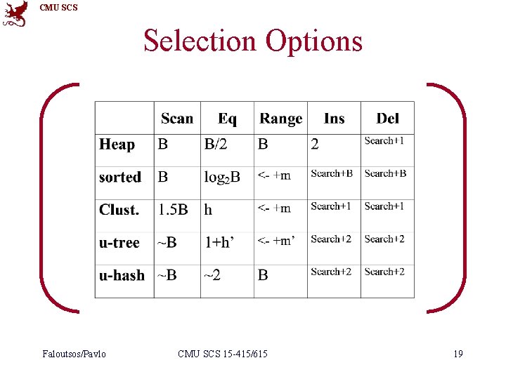
CMU SCS Selection Options Faloutsos/Pavlo CMU SCS 15 -415/615 19

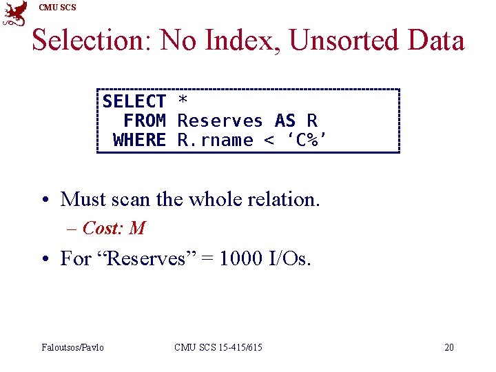
CMU SCS Selection: No Index, Unsorted Data SELECT * FROM Reserves AS R WHERE R. rname < ‘C%’ • Must scan the whole relation. – Cost: M • For “Reserves” = 1000 I/Os. Faloutsos/Pavlo CMU SCS 15 -415/615 20

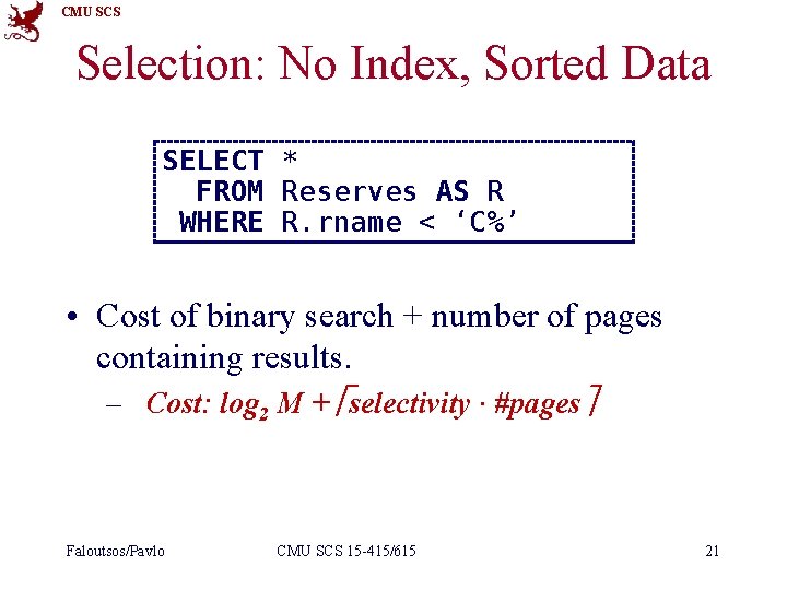
CMU SCS Selection: No Index, Sorted Data SELECT * FROM Reserves AS R WHERE R. rname < ‘C%’ • Cost of binary search + number of pages containing results. – Cost: log 2 M + selectivity ∙ #pages Faloutsos/Pavlo CMU SCS 15 -415/615 21

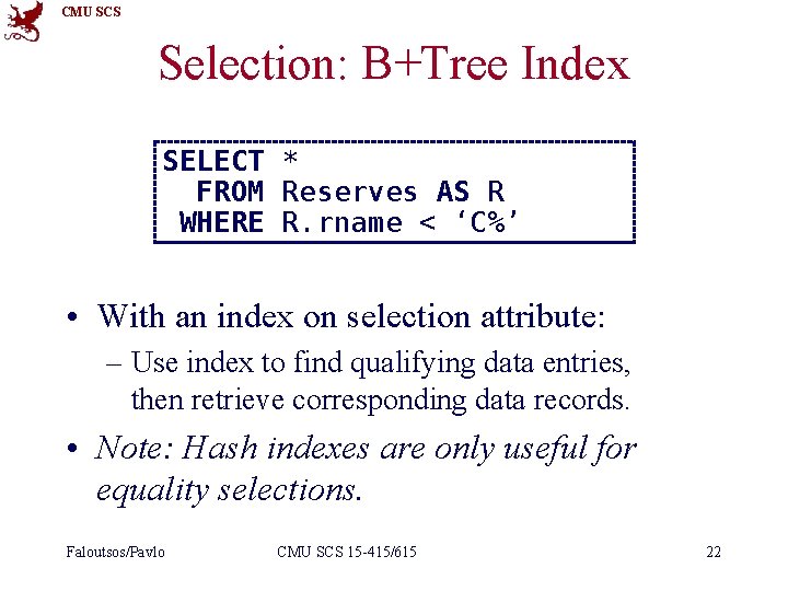
CMU SCS Selection: B+Tree Index SELECT * FROM Reserves AS R WHERE R. rname < ‘C%’ • With an index on selection attribute: – Use index to find qualifying data entries, then retrieve corresponding data records. • Note: Hash indexes are only useful for equality selections. Faloutsos/Pavlo CMU SCS 15 -415/615 22

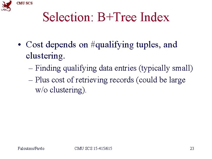
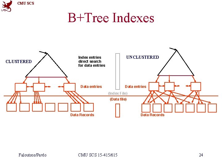
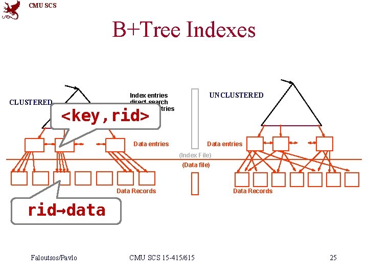
CMU SCS Selection: B+Tree Index • Cost depends on #qualifying tuples, and clustering. – Finding qualifying data entries (typically small) – Plus cost of retrieving records (could be large w/o clustering). Faloutsos/Pavlo CMU SCS 15 -415/615 23

CMU SCS B+Tree Indexes CLUSTERED UNCLUSTERED Index entries direct search for data entries Data entries (Index File) (Data file) Data Records Faloutsos/Pavlo CMU SCS 15 -415/615 Data Records 24

CMU SCS B+Tree Indexes CLUSTERED UNCLUSTERED Index entries direct search for data entries <key, rid> Data entries (Index File) (Data file) Data Records rid→data Faloutsos/Pavlo CMU SCS 15 -415/615 25

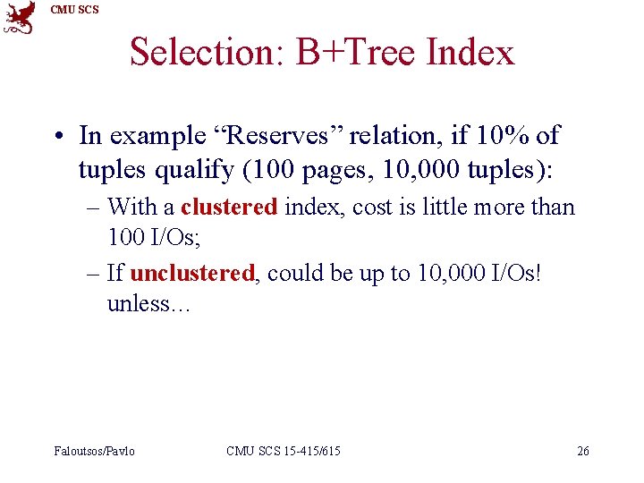
CMU SCS Selection: B+Tree Index • In example “Reserves” relation, if 10% of tuples qualify (100 pages, 10, 000 tuples): – With a clustered index, cost is little more than 100 I/Os; – If unclustered, could be up to 10, 000 I/Os! unless… Faloutsos/Pavlo CMU SCS 15 -415/615 26

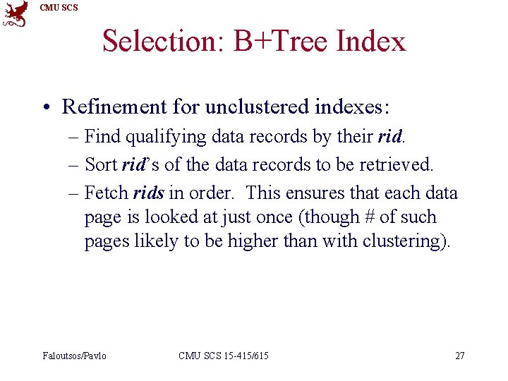
CMU SCS Selection: B+Tree Index • Refinement for unclustered indexes: – Find qualifying data records by their rid. – Sort rid’s of the data records to be retrieved. – Fetch rids in order. This ensures that each data page is looked at just once (though # of such pages likely to be higher than with clustering). Faloutsos/Pavlo CMU SCS 15 -415/615 27

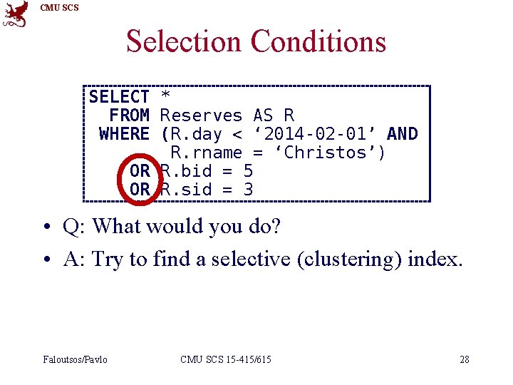
CMU SCS Selection Conditions SELECT * FROM Reserves AS R WHERE (R. day < ‘ 2014 -02 -01’ AND R. rname = ‘Christos’) OR R. bid = 5 OR R. sid = 3 • Q: What would you do? • A: Try to find a selective (clustering) index. Faloutsos/Pavlo CMU SCS 15 -415/615 28

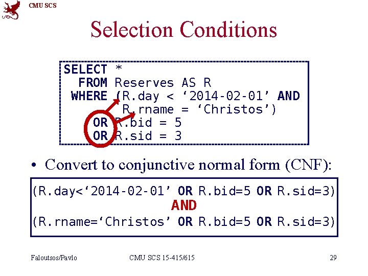
CMU SCS Selection Conditions SELECT * FROM Reserves AS R WHERE (R. day < ‘ 2014 -02 -01’ AND R. rname = ‘Christos’) OR R. bid = 5 OR R. sid = 3 • Convert to conjunctive normal form (CNF): (R. day<‘ 2014 -02 -01’ OR R. bid=5 OR R. sid=3) AND (R. rname=‘Christos’ OR R. bid=5 OR R. sid=3) Faloutsos/Pavlo CMU SCS 15 -415/615 29

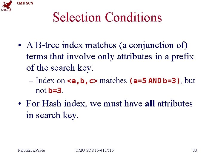
CMU SCS Selection Conditions • A B-tree index matches (a conjunction of) terms that involve only attributes in a prefix of the search key. – Index on <a, b, c> matches (a=5 AND b=3), but not b=3. • For Hash index, we must have all attributes in search key. Faloutsos/Pavlo CMU SCS 15 -415/615 30

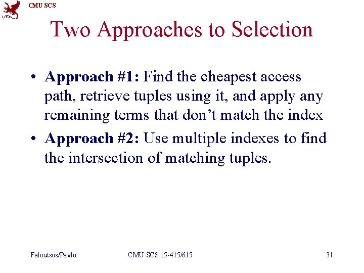
CMU SCS Two Approaches to Selection • Approach #1: Find the cheapest access path, retrieve tuples using it, and apply any remaining terms that don’t match the index • Approach #2: Use multiple indexes to find the intersection of matching tuples. Faloutsos/Pavlo CMU SCS 15 -415/615 31

CMU SCS Approach #1 • Find the cheapest access path, retrieve tuples using it, and apply any remaining terms that don’t match the index: – Cheapest access path: An index or file scan with fewest I/Os. – Terms that match this index reduce the number of tuples retrieved; other terms help discard some retrieved tuples, but do not affect number of tuples/pages fetched. Faloutsos/Pavlo CMU SCS 15 -415/615 32

CMU SCS Approach #1 – Example (day<‘ 2014 -02 -01’ AND bid=5 AND sid=3) • A B+ tree index on day can be used; – then, bid=5 and sid=3 must be checked for each retrieved tuple. • Similarly, a hash index on <bid, sid> could be used; – Then, day<‘ 2014 -02 -01’ must be checked. Faloutsos/Pavlo CMU SCS 15 -415/615 33

CMU SCS Approach #1 – Example (day<‘ 2014 -02 -01’ AND bid=5 AND sid=3) • How about a B+tree on <rname, day>? • How about a B+tree on <day, rname>? • How about a Hash index on <day, rname>? What if we have multiple indexes? Faloutsos/Pavlo CMU SCS 15 -415/615 34

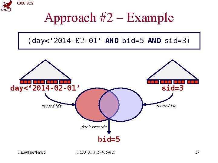
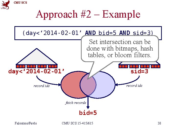
CMU SCS Approach #2 • Get rids from first index; rids from second index; intersect and fetch. • If we have 2 or more matching indexes: – Get sets of rids of data records using each matching index. – Then intersect these sets of rids. – Retrieve the records and apply any remaining terms. Faloutsos/Pavlo CMU SCS 15 -415/615 35

CMU SCS Approach #2 – Example (day<‘ 2014 -02 -01’ AND bid=5 AND sid=3) • With a B+ tree index on day and an index on sid, – We can retrieve rids of records satisfying day<‘ 2014 -02 -01’ using the first, – rids of recs satisfying sid=3 using the second, – intersect, – retrieve records and check bid=5. Faloutsos/Pavlo CMU SCS 15 -415/615 36

CMU SCS Approach #2 – Example (day<‘ 2014 -02 -01’ AND bid=5 AND sid=3) day<‘ 2014 -02 -01’ sid=3 record ids fetch records bid=5 Faloutsos/Pavlo CMU SCS 15 -415/615 37

CMU SCS Approach #2 – Example (day<‘ 2014 -02 -01’ AND bid=5 AND sid=3) Set intersection can be done with bitmaps, hash tables, or bloom filters. day<‘ 2014 -02 -01’ sid=3 record ids fetch records bid=5 Faloutsos/Pavlo CMU SCS 15 -415/615 38

CMU SCS Summary • For selections, we always want an index. – B+Trees are more versatile. – Hash indexes are faster, but only support equality predicates. • Last resort is to just scan entire table. Faloutsos/Pavlo CMU SCS 15 -415/615 39

CMU SCS Today’s Class • Introduction • Selection • Joins Faloutsos/Pavlo CMU SCS 15 -415/615 40

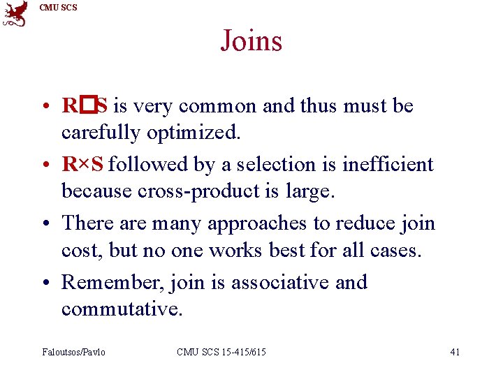
CMU SCS Joins • R�S is very common and thus must be carefully optimized. • R×S followed by a selection is inefficient because cross-product is large. • There are many approaches to reduce join cost, but no one works best for all cases. • Remember, join is associative and commutative. Faloutsos/Pavlo CMU SCS 15 -415/615 41

CMU SCS Faloutsos/Pavlo CMU SCS 15 -415/615 42

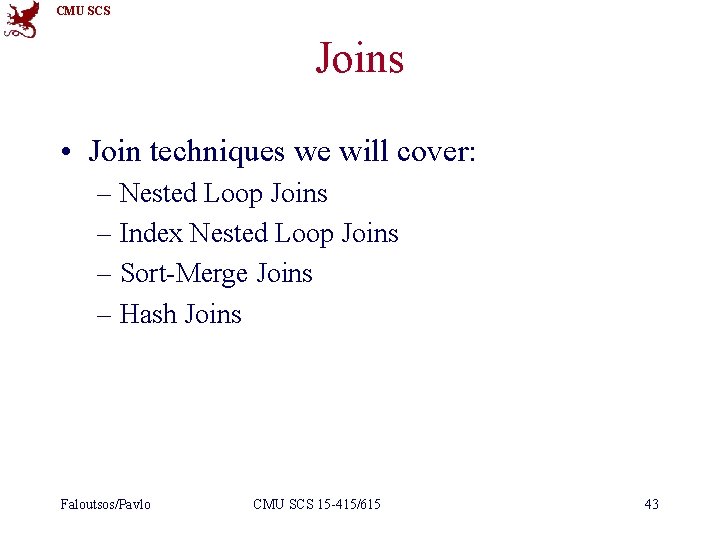
CMU SCS Joins • Join techniques we will cover: – Nested Loop Joins – Index Nested Loop Joins – Sort-Merge Joins – Hash Joins Faloutsos/Pavlo CMU SCS 15 -415/615 43

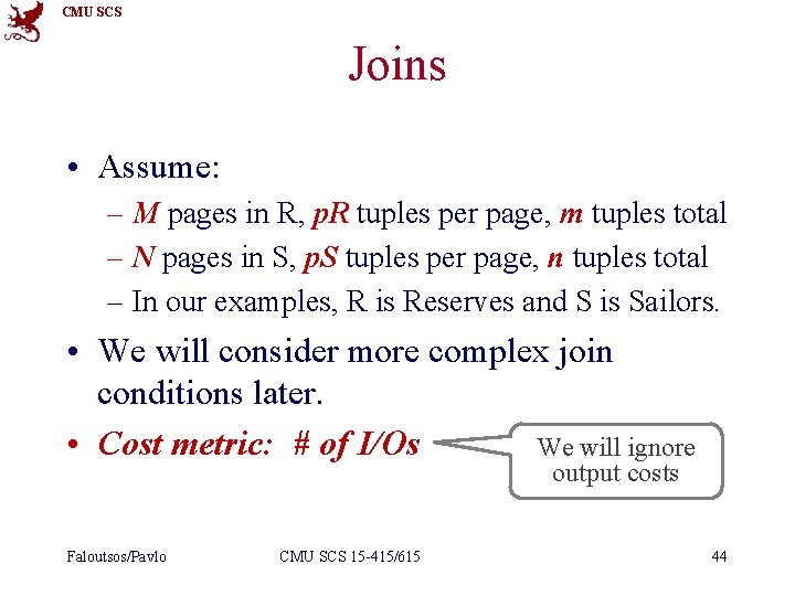
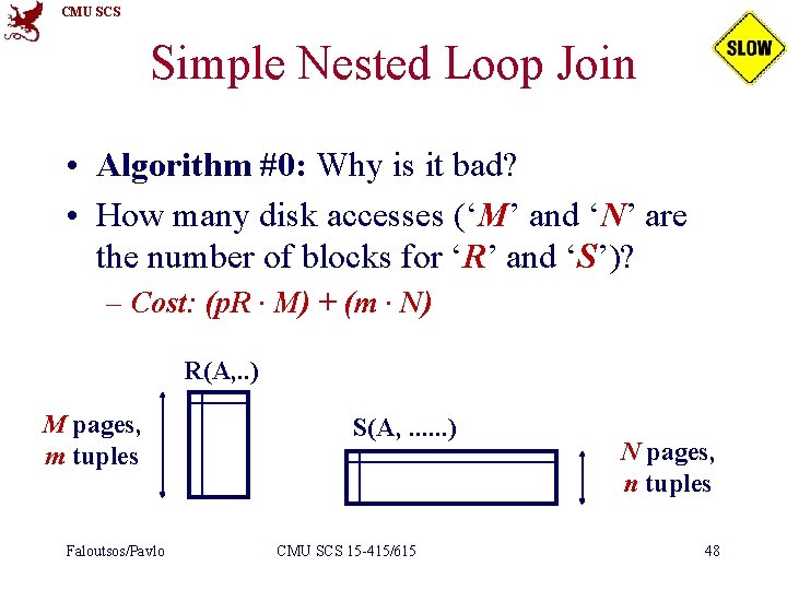
CMU SCS Joins • Assume: – M pages in R, p. R tuples per page, m tuples total – N pages in S, p. S tuples per page, n tuples total – In our examples, R is Reserves and S is Sailors. • We will consider more complex join conditions later. • Cost metric: # of I/Os We will ignore output costs Faloutsos/Pavlo CMU SCS 15 -415/615 44

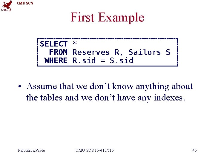
CMU SCS First Example SELECT * FROM Reserves R, Sailors S WHERE R. sid = S. sid • Assume that we don’t know anything about the tables and we don’t have any indexes. Faloutsos/Pavlo CMU SCS 15 -415/615 45

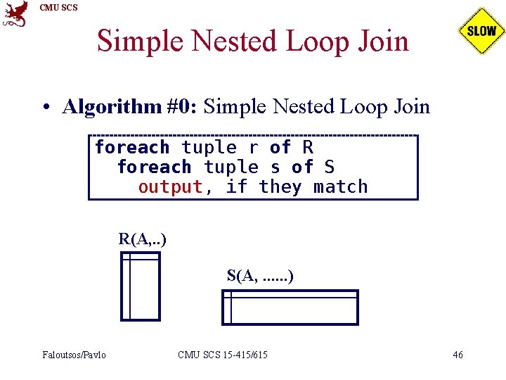
CMU SCS Simple Nested Loop Join • Algorithm #0: Simple Nested Loop Join foreach tuple r of R foreach tuple s of S output, if they match R(A, . . ) S(A, . . . ) Faloutsos/Pavlo CMU SCS 15 -415/615 46

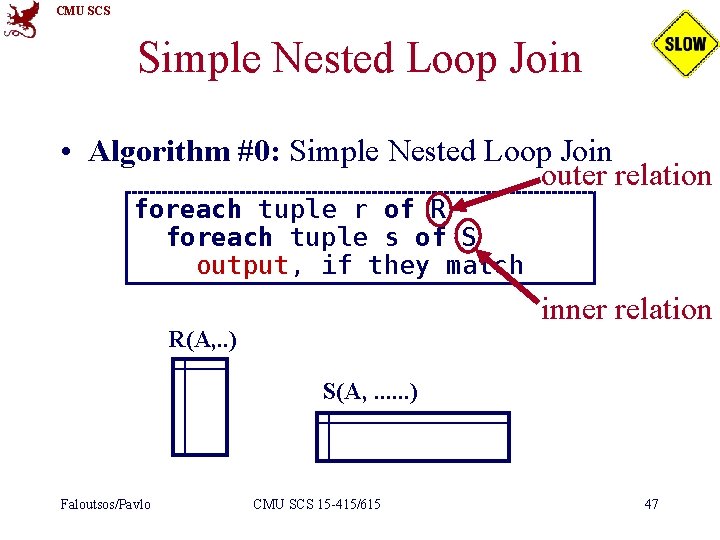
CMU SCS Simple Nested Loop Join • Algorithm #0: Simple Nested Loop Join outer relation foreach tuple r of R foreach tuple s of S output, if they match inner relation R(A, . . ) S(A, . . . ) Faloutsos/Pavlo CMU SCS 15 -415/615 47

CMU SCS Simple Nested Loop Join • Algorithm #0: Why is it bad? • How many disk accesses (‘M’ and ‘N’ are the number of blocks for ‘R’ and ‘S’)? – Cost: (p. R ∙ M) + (m ∙ N) R(A, . . ) M pages, m tuples Faloutsos/Pavlo S(A, . . . ) CMU SCS 15 -415/615 N pages, n tuples 48

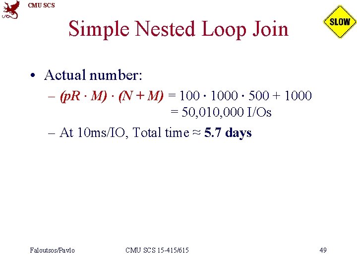
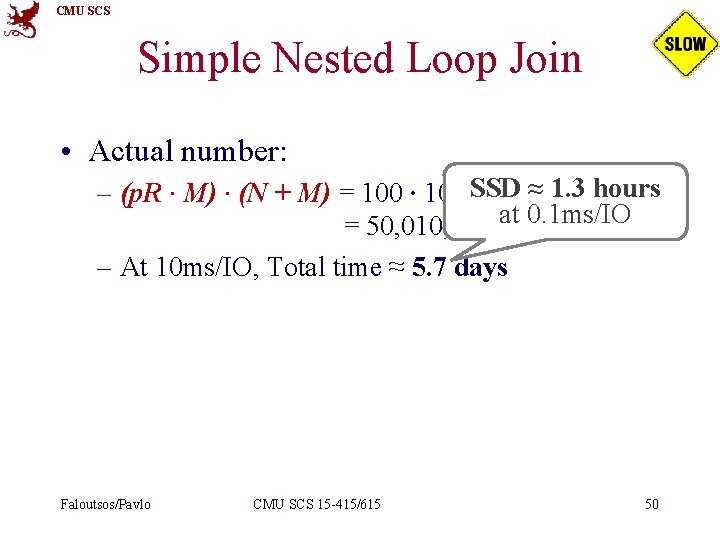
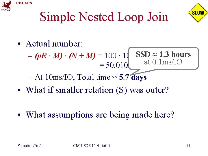
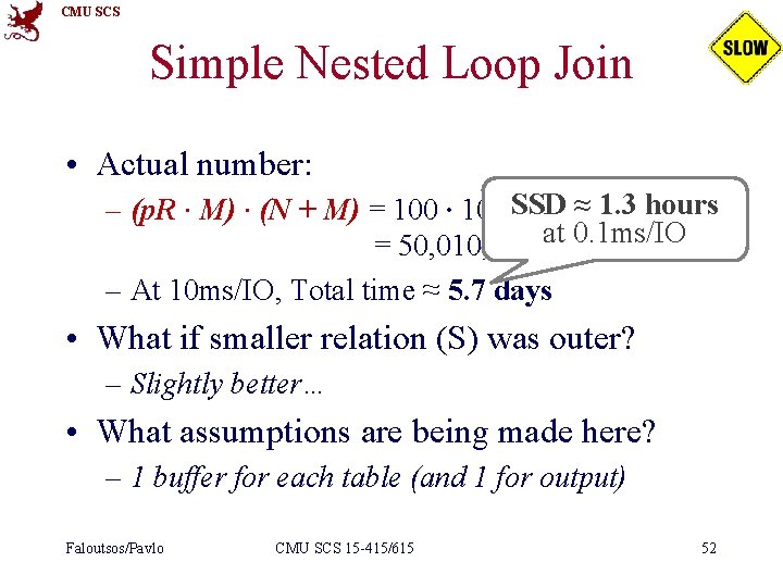
CMU SCS Simple Nested Loop Join • Actual number: – (p. R ∙ M) ∙ (N + M) = 100 ∙ 1000 ∙ 500 + 1000 = 50, 010, 000 I/Os – At 10 ms/IO, Total time ≈ 5. 7 days • What if smaller relation (S) was outer? – Slightly better… • What assumptions are being made here? – 1 buffer for each table (and 1 for output) Faloutsos/Pavlo CMU SCS 15 -415/615 49

CMU SCS Simple Nested Loop Join • Actual number: ≈+ 1. 31000 hours – (p. R ∙ M) ∙ (N + M) = 100 ∙ 1000 SSD ∙ 500 0. 1 ms/IO = 50, 010, 000 at I/Os – At 10 ms/IO, Total time ≈ 5. 7 days • What if smaller relation (S) was outer? – Slightly better… • What assumptions are being made here? – 1 buffer for each table (and 1 for output) Faloutsos/Pavlo CMU SCS 15 -415/615 50

CMU SCS Simple Nested Loop Join • Actual number: ≈+ 1. 31000 hours – (p. R ∙ M) ∙ (N + M) = 100 ∙ 1000 SSD ∙ 500 0. 1 ms/IO = 50, 010, 000 at I/Os – At 10 ms/IO, Total time ≈ 5. 7 days • What if smaller relation (S) was outer? – Slightly better… • What assumptions are being made here? – 1 buffer for each table (and 1 for output) Faloutsos/Pavlo CMU SCS 15 -415/615 51

CMU SCS Simple Nested Loop Join • Actual number: ≈+ 1. 31000 hours – (p. R ∙ M) ∙ (N + M) = 100 ∙ 1000 SSD ∙ 500 0. 1 ms/IO = 50, 010, 000 at I/Os – At 10 ms/IO, Total time ≈ 5. 7 days • What if smaller relation (S) was outer? – Slightly better… • What assumptions are being made here? – 1 buffer for each table (and 1 for output) Faloutsos/Pavlo CMU SCS 15 -415/615 52

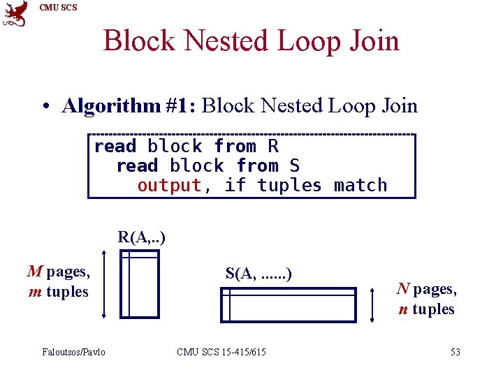
CMU SCS Block Nested Loop Join • Algorithm #1: Block Nested Loop Join read block from R read block from S output, if tuples match R(A, . . ) M pages, m tuples Faloutsos/Pavlo S(A, . . . ) CMU SCS 15 -415/615 N pages, n tuples 53

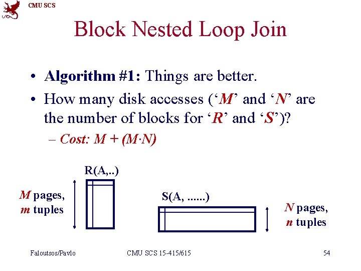
CMU SCS Block Nested Loop Join • Algorithm #1: Things are better. • How many disk accesses (‘M’ and ‘N’ are the number of blocks for ‘R’ and ‘S’)? – Cost: M + (M∙N) R(A, . . ) M pages, m tuples Faloutsos/Pavlo S(A, . . . ) CMU SCS 15 -415/615 N pages, n tuples 54

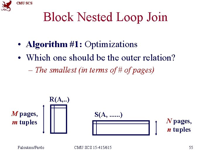
CMU SCS Block Nested Loop Join • Algorithm #1: Optimizations • Which one should be the outer relation? – The smallest (in terms of # of pages) R(A, . . ) M pages, m tuples Faloutsos/Pavlo S(A, . . . ) CMU SCS 15 -415/615 N pages, n tuples 55

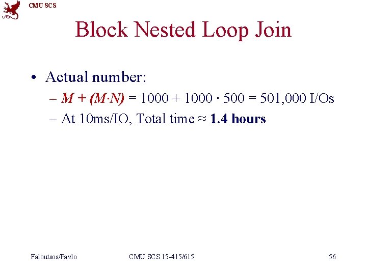
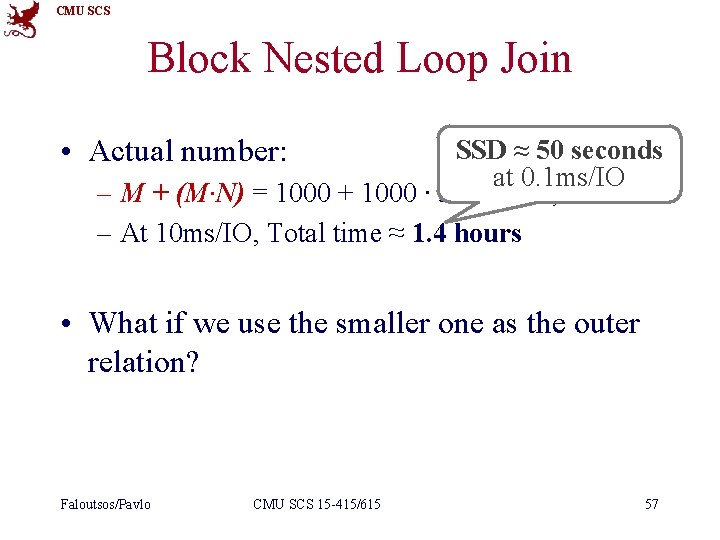
CMU SCS Block Nested Loop Join • Actual number: – M + (M∙N) = 1000 + 1000 ∙ 500 = 501, 000 I/Os – At 10 ms/IO, Total time ≈ 1. 4 hours Faloutsos/Pavlo CMU SCS 15 -415/615 56

CMU SCS Block Nested Loop Join • Actual number: SSD ≈ 50 seconds at 0. 1 ms/IO – M + (M∙N) = 1000 + 1000 ∙ 500 = 501, 000 I/Os – At 10 ms/IO, Total time ≈ 1. 4 hours • What if we use the smaller one as the outer relation? Faloutsos/Pavlo CMU SCS 15 -415/615 57

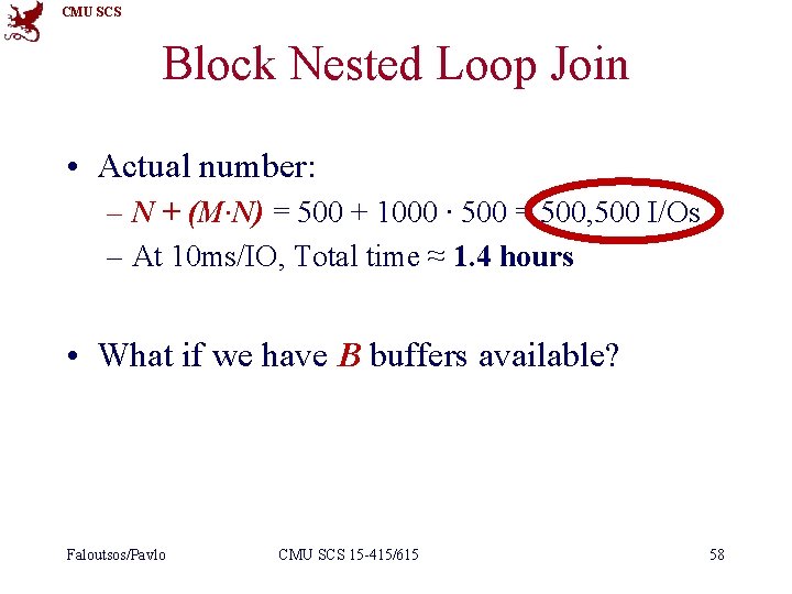
CMU SCS Block Nested Loop Join • Actual number: – N + (M∙N) = 500 + 1000 ∙ 500 = 500, 500 I/Os – At 10 ms/IO, Total time ≈ 1. 4 hours • What if we have B buffers available? – Give B-2 buffers to outer relation, 1 to inner relation, 1 for output Faloutsos/Pavlo CMU SCS 15 -415/615 58

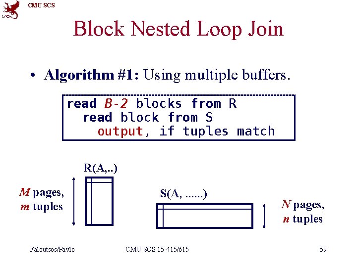
CMU SCS Block Nested Loop Join • Algorithm #1: Using multiple buffers. read B-2 blocks from R read block from S output, if tuples match R(A, . . ) M pages, m tuples Faloutsos/Pavlo S(A, . . . ) CMU SCS 15 -415/615 N pages, n tuples 59

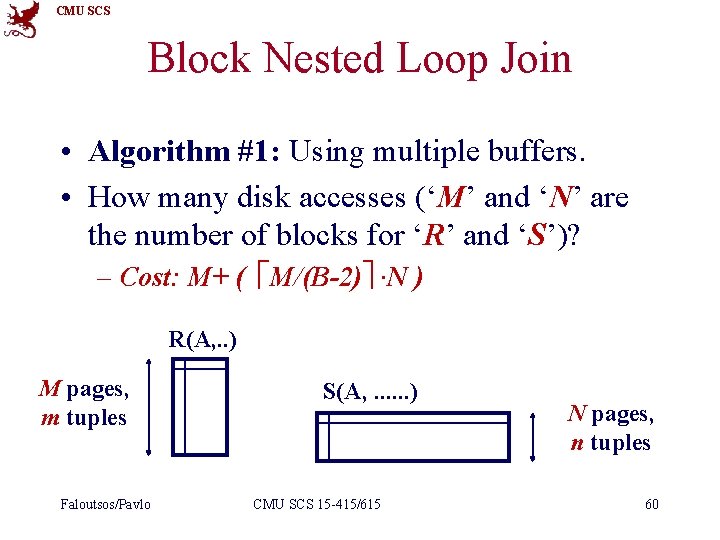
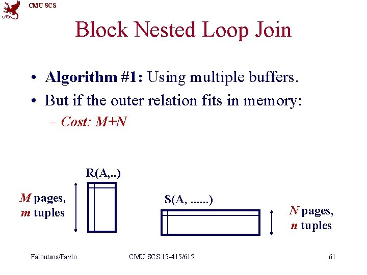
CMU SCS Block Nested Loop Join • Algorithm #1: Using multiple buffers. • How many disk accesses (‘M’ and ‘N’ are the number of blocks for ‘R’ and ‘S’)? – Cost: M+ ( M/(B-2) ∙N ) R(A, . . ) M pages, m tuples Faloutsos/Pavlo S(A, . . . ) CMU SCS 15 -415/615 N pages, n tuples 60

CMU SCS Block Nested Loop Join • Algorithm #1: Using multiple buffers. • But if the outer relation fits in memory: – Cost: M+N R(A, . . ) M pages, m tuples Faloutsos/Pavlo S(A, . . . ) CMU SCS 15 -415/615 N pages, n tuples 61

CMU SCS Joins • Join techniques we will cover: – Nested Loop Joins – Index Nested Loop Joins – Sort-Merge Joins – Hash Joins Faloutsos/Pavlo CMU SCS 15 -415/615 62

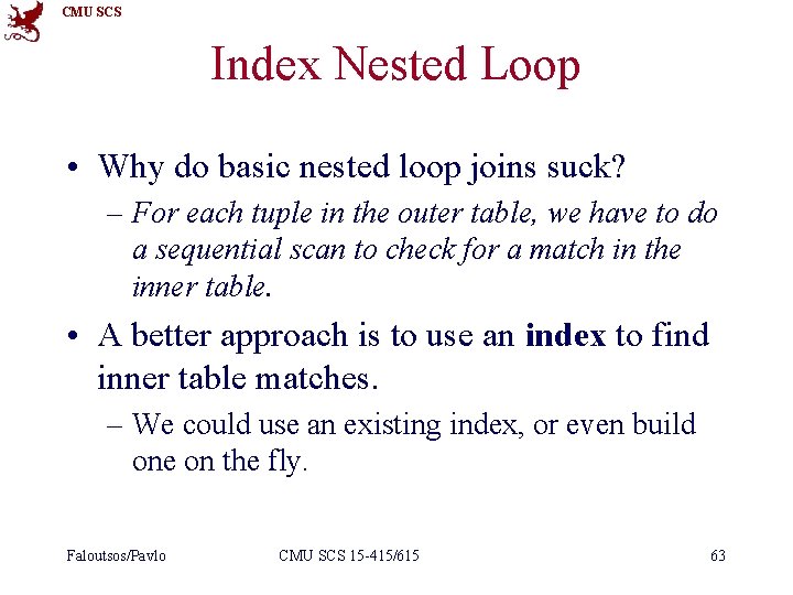
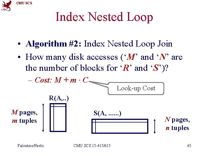
CMU SCS Index Nested Loop • Why do basic nested loop joins suck? – For each tuple in the outer table, we have to do a sequential scan to check for a match in the inner table. • A better approach is to use an index to find inner table matches. – We could use an existing index, or even build one on the fly. Faloutsos/Pavlo CMU SCS 15 -415/615 63

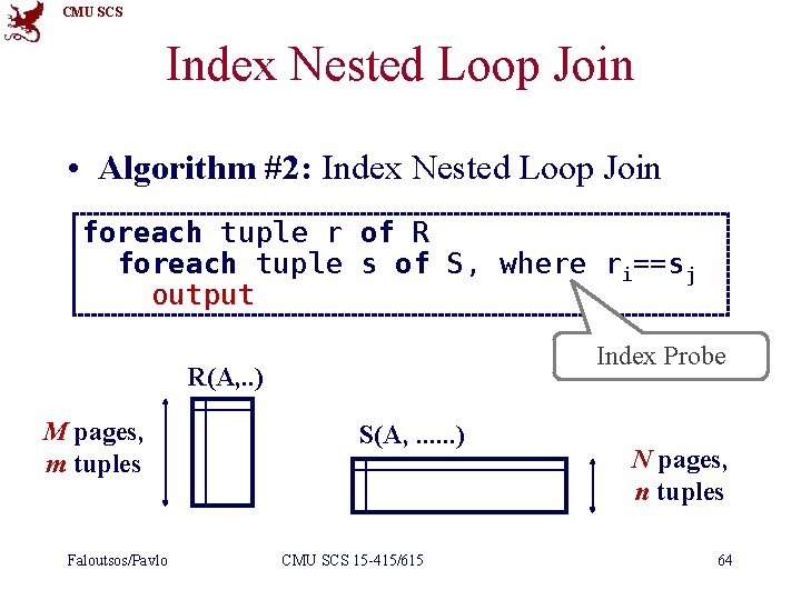
CMU SCS Index Nested Loop Join • Algorithm #2: Index Nested Loop Join foreach tuple r of R foreach tuple s of S, where ri==sj output Index Probe R(A, . . ) M pages, m tuples Faloutsos/Pavlo S(A, . . . ) CMU SCS 15 -415/615 N pages, n tuples 64

CMU SCS Index Nested Loop • Algorithm #2: Index Nested Loop Join • How many disk accesses (‘M’ and ‘N’ are the number of blocks for ‘R’ and ‘S’)? – Cost: M + m ∙ C Look-up Cost R(A, . . ) M pages, m tuples Faloutsos/Pavlo S(A, . . . ) CMU SCS 15 -415/615 N pages, n tuples 65

CMU SCS Nested Loop Joins Guideline • Pick the smallest table as the outer relation – i. e. , the one with the fewest pages • Put as much of it in memory as possible • Loop over the inner Faloutsos/Pavlo CMU SCS 15 -415/615 66

CMU SCS Joins • Join techniques we will cover: – Nested Loop Joins – Index Nested Loop Joins – Sort-Merge Joins – Hash Joins Faloutsos/Pavlo CMU SCS 15 -415/615 67

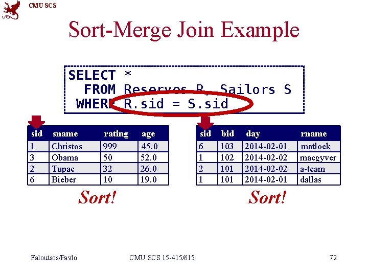
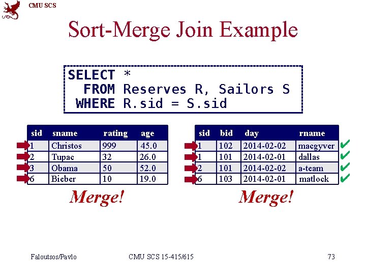
CMU SCS Sort-Merge Join • First sort both tables on joining attribute. • Then step through each one in lock-step to find matches. Faloutsos/Pavlo CMU SCS 15 -415/615 68

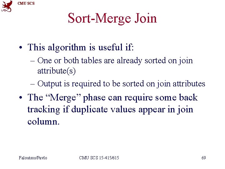
CMU SCS Sort-Merge Join • This algorithm is useful if: – One or both tables are already sorted on join attribute(s) – Output is required to be sorted on join attributes • The “Merge” phase can require some back tracking if duplicate values appear in join column. Faloutsos/Pavlo CMU SCS 15 -415/615 69

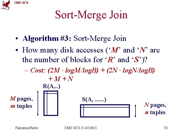
CMU SCS Sort-Merge Join • Algorithm #3: Sort-Merge Join • How many disk accesses (‘M’ and ‘N’ are the number of blocks for ‘R’ and ‘S’)? – Cost: (2 M ∙ log. M/log. B) + (2 N ∙ log. N/log. B) +M+N R(A, . . ) M pages, m tuples Faloutsos/Pavlo S(A, . . . ) CMU SCS 15 -415/615 N pages, n tuples 70

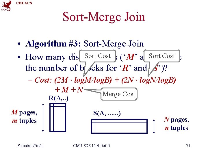
CMU SCS Sort-Merge Join • Algorithm #3: Sort-Merge Join Cost (‘M’ and Sort Cost • How many disk Sort accesses ‘N’ are the number of blocks for ‘R’ and ‘S’)? – Cost: (2 M ∙ log. M/log. B) + (2 N ∙ log. N/log. B) +M+N Merge Cost R(A, . . ) M pages, m tuples Faloutsos/Pavlo S(A, . . . ) CMU SCS 15 -415/615 N pages, n tuples 71

CMU SCS Sort-Merge Join Example SELECT * FROM Reserves R, Sailors S WHERE R. sid = S. sid 1 3 2 6 sname Christos Obama Tupac Bieber rating 999 50 32 10 age 45. 0 52. 0 26. 0 19. 0 Sort! Faloutsos/Pavlo sid 6 1 2 1 bid 103 102 101 day 2014 -02 -01 2014 -02 -02 2014 -02 -01 rname matlock macgyver a-team dallas Sort! CMU SCS 15 -415/615 72

CMU SCS Sort-Merge Join Example SELECT * FROM Reserves R, Sailors S WHERE R. sid = S. sid 1 2 3 6 sname Christos Tupac Obama Bieber rating 999 32 50 10 age 45. 0 26. 0 52. 0 19. 0 Merge! Faloutsos/Pavlo sid 1 1 2 6 bid 102 101 103 day 2014 -02 -02 2014 -02 -01 rname macgyver dallas a-team matlock Merge! CMU SCS 15 -415/615 73 ✔ ✔

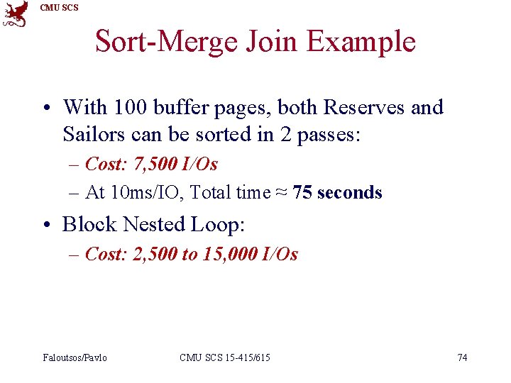
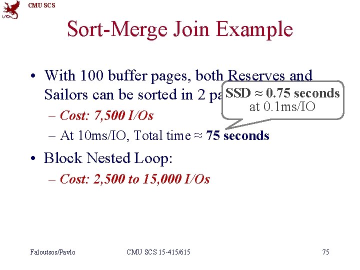
CMU SCS Sort-Merge Join Example • With 100 buffer pages, both Reserves and Sailors can be sorted in 2 passes: – Cost: 7, 500 I/Os – At 10 ms/IO, Total time ≈ 75 seconds • Block Nested Loop: – Cost: 2, 500 to 15, 000 I/Os Faloutsos/Pavlo CMU SCS 15 -415/615 74

CMU SCS Sort-Merge Join Example • With 100 buffer pages, both Reserves and SSD ≈ 0. 75 seconds Sailors can be sorted in 2 passes: at 0. 1 ms/IO – Cost: 7, 500 I/Os – At 10 ms/IO, Total time ≈ 75 seconds • Block Nested Loop: – Cost: 2, 500 to 15, 000 I/Os Faloutsos/Pavlo CMU SCS 15 -415/615 75

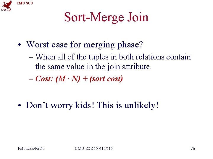
CMU SCS Sort-Merge Join • Worst case for merging phase? – When all of the tuples in both relations contain the same value in the join attribute. – Cost: (M ∙ N) + (sort cost) • Don’t worry kids! This is unlikely! Faloutsos/Pavlo CMU SCS 15 -415/615 76

CMU SCS Sort-Merge Join Optimizations • All the refinements from external sorting • Plus overlapping of the merging of sorting with the merging of joining. Faloutsos/Pavlo CMU SCS 15 -415/615 77

CMU SCS Joins • Join techniques we will cover: – Nested Loop Joins – Index Nested Loop Joins – Sort-Merge Joins – Hash Joins Faloutsos/Pavlo CMU SCS 15 -415/615 78

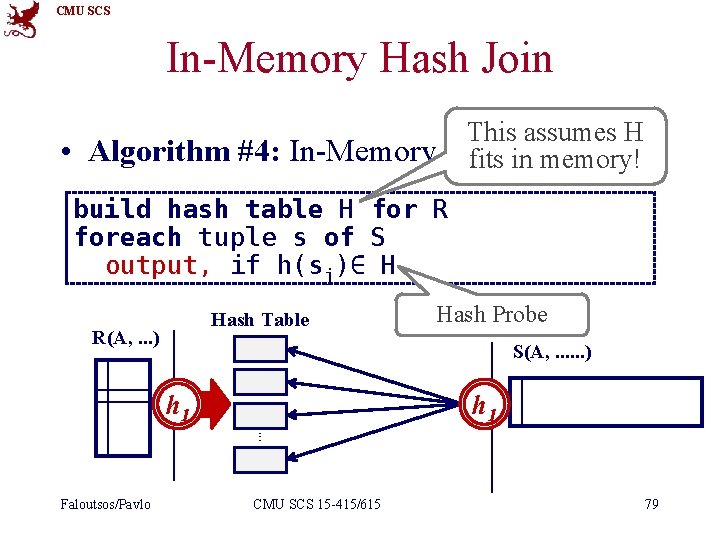
CMU SCS In-Memory Hash Join This assumes H • Algorithm #4: In-Memory Hash Join fits in memory! build hash table H for R foreach tuple s of S output, if h(sj)∈ H Hash Table R(A, . . . ) Hash Probe S(A, . . . ) h 1 ⋮ Faloutsos/Pavlo CMU SCS 15 -415/615 79

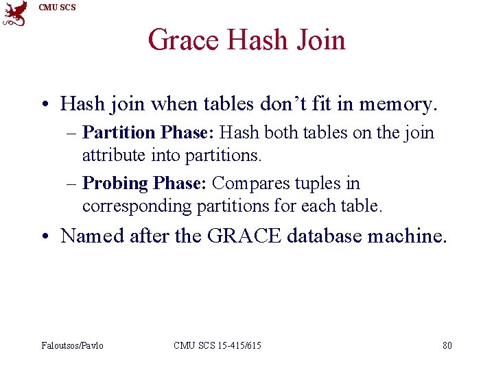
CMU SCS Grace Hash Join • Hash join when tables don’t fit in memory. – Partition Phase: Hash both tables on the join attribute into partitions. – Probing Phase: Compares tuples in corresponding partitions for each table. • Named after the GRACE database machine. Faloutsos/Pavlo CMU SCS 15 -415/615 80

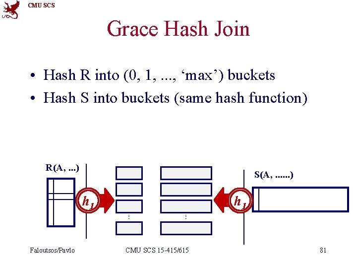
CMU SCS Grace Hash Join • Hash R into (0, 1, . . . , ‘max’) buckets • Hash S into buckets (same hash function) R(A, . . . ) S(A, . . . ) h 1 ⋮ Faloutsos/Pavlo ⋮ CMU SCS 15 -415/615 81

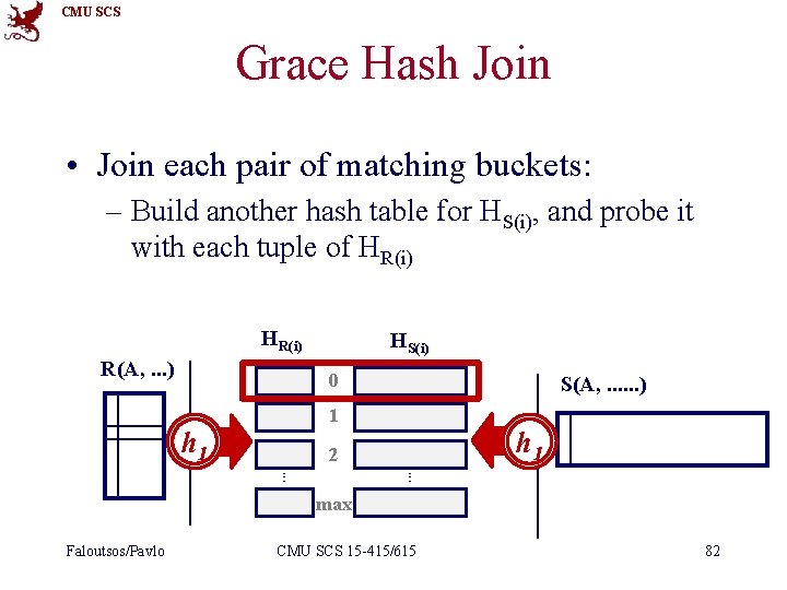
CMU SCS Grace Hash Join • Join each pair of matching buckets: – Build another hash table for HS(i), and probe it with each tuple of HR(i) R(A, . . . ) HS(i) 0 S(A, . . . ) 1 h 1 2 ⋮ ⋮ max Faloutsos/Pavlo CMU SCS 15 -415/615 82

CMU SCS Grace Hash Join • Choose the (page-wise) smallest - if it fits in memory, do a nested loop join – Build a hash table (with h 2() != h()) – And then probe it for each tuple of the other Faloutsos/Pavlo CMU SCS 15 -415/615 83

CMU SCS Grace Hash Join • What if HS(i) is too large to fit in memory? – Recursive Partitioning! – More details (overflows, hybrid hash joins) available in textbook (Ch 14. 4. 3) Faloutsos/Pavlo CMU SCS 15 -415/615 84

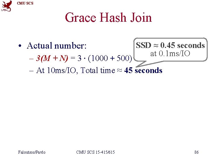
CMU SCS Grace Hash Join • Cost of hash join? – Assume that we have enough buffers. – Cost: 3(M + N) • Partitioning Phase: read+write both tables – 2(M+N) I/Os • Probing Phase: read both tables – M+N I/Os Faloutsos/Pavlo CMU SCS 15 -415/615 85

CMU SCS Grace Hash Join • Actual number: SSD ≈ 0. 45 seconds at 0. 1 ms/IO – 3(M + N) = 3 ∙ (1000 + 500) = 4, 500 I/Os – At 10 ms/IO, Total time ≈ 45 seconds Faloutsos/Pavlo CMU SCS 15 -415/615 86

CMU SCS Sort-Merge Join vs. Hash Join • Given a minimum amount of memory both have a cost of 3(M+N) I/Os. • When do we want to choose one over the other? Faloutsos/Pavlo CMU SCS 15 -415/615 87

CMU SCS Sort-Merge Join vs. Hash Join • Sort-Merge: – Less sensitive to data skew. – Result is sorted (may help upstream operators). – Goes faster if one or both inputs already sorted. • Hash: – Superior if relation sizes differ greatly. – Shown to be highly. Faloutsos/Pavlo CMU SCS 15 -415/615 88

CMU SCS Sort-Merge Join vs. Hash Join • Sort-Merge: – Less sensitive to data skew. – Result is sorted (may help upstream operators). – Goes faster if one or both inputs already sorted. • Hash: – Superior if relation sizes differ greatly. – Shown to be highly. Faloutsos/Pavlo CMU SCS 15 -415/615 89

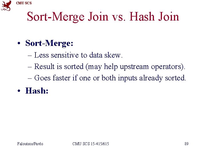
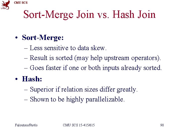
CMU SCS Sort-Merge Join vs. Hash Join • Sort-Merge: – Less sensitive to data skew. – Result is sorted (may help upstream operators). – Goes faster if one or both inputs already sorted. • Hash: – Superior if relation sizes differ greatly. – Shown to be highly parallelizable. Faloutsos/Pavlo CMU SCS 15 -415/615 90

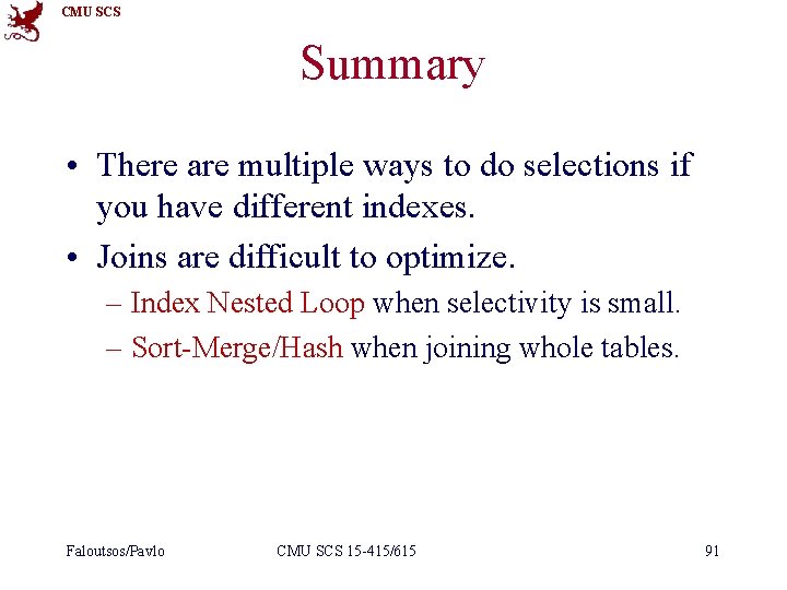
CMU SCS Summary • There are multiple ways to do selections if you have different indexes. • Joins are difficult to optimize. – Index Nested Loop when selectivity is small. – Sort-Merge/Hash when joining whole tables. Faloutsos/Pavlo CMU SCS 15 -415/615 91

CMU SCS Next Class • Set & Aggregate Operations • Query Optimizations • Brief Midterm Review Faloutsos/Pavlo CMU SCS 15 -415/615 92