CMSC 100 Heuristic Search and Game Playing Professor

CMSC 100 Heuristic Search and Game Playing Professor Marie des. Jardins Tuesday, November 13, 2012 E-Commerce and Databases 1 Thu 10/25/12

Summary of Topics n What is heuristic search? n Examples of search problems n Search methods n Uninformed search n Informed search n Local search n Game trees 2

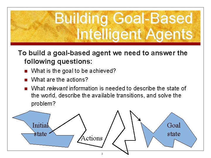
Building Goal-Based Intelligent Agents To build a goal-based agent we need to answer the following questions: n n n What is the goal to be achieved? What are the actions? What relevant information is needed to describe the state of the world, describe the available transitions, and solve the problem? Initial state Actions 3 Goal state

Representing States n What information is needed to sufficiently describe all relevant aspects to solving the goal? n n That is, what knowledge needs to be represented in a state description to adequately describe the current state or situation of the world? The size of a problem is usually described in terms of the number of states that are possible. n Tic-Tac-Toe has about 39 states. n Checkers has about 1040 states. n Rubik’s Cube has about 1019 states. n Chess has about 10120 states in a typical game. 4

Real-world Search Problems n Route finding (GPS algorithms, Google Maps) n Touring (traveling salesman) n Logistics n VLSI layout n Robot navigation n Learning 5

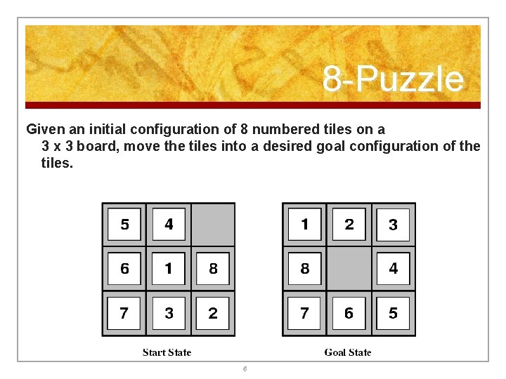
8 -Puzzle Given an initial configuration of 8 numbered tiles on a 3 x 3 board, move the tiles into a desired goal configuration of the tiles. 6

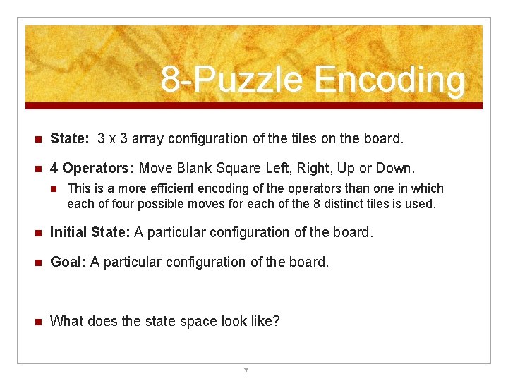
8 -Puzzle Encoding n State: 3 x 3 array configuration of the tiles on the board. n 4 Operators: Move Blank Square Left, Right, Up or Down. n This is a more efficient encoding of the operators than one in which each of four possible moves for each of the 8 distinct tiles is used. n Initial State: A particular configuration of the board. n Goal: A particular configuration of the board. n What does the state space look like? 7

Solution Cost n A solution is a sequence of operators that is associated with a path in a state space from a start node to a goal node. n The cost of a solution is the sum of the arc costs on the solution path. n If all arcs have the same (unit) cost, then the solution cost is just the length of the solution (number of steps / state transitions) 8

Evaluating Search Strategies n Completeness n n Time complexity n n How long (worst or average case) does it take to find a solution? Usually measured in terms of the number of nodes expanded Space complexity n n Guarantees finding a solution whenever one exists How much space is used by the algorithm? Usually measured in terms of the maximum size of the “nodes” list during the search Optimality/Admissibility n If a solution is found, is it guaranteed to be an optimal one? That is, is it the one with minimum cost? 9

Search Methods n Uninformed search strategies n n Also known as “blind search, ” uninformed search strategies use no information about the likely “direction” of the goal node(s) Variations on “generate and test” or “trial and error” approach Uninformed search methods: breadth-first, depth-first, uniform-cost Informed search strategies n n n Also known as “heuristic search, ” informed search strategies use information about the domain to (try to) (usually) head in the general direction of the goal node(s) Informed search methods: greedy search, (A*) (Informed search is what your GPS does!!) 10

Search Methods cont. n Local search strategies n n n Pick a starting solution (that might not be very good) and incrementally try to improve it Local search methods: hill-climbing, genetic algorithms Game trees n n Search strategies for situations where you have an opponent who gets to make some of the moves Try to pick moves that will let you win most of the time by “looking ahead” to see what your opponent might do 11

Uninformed Search

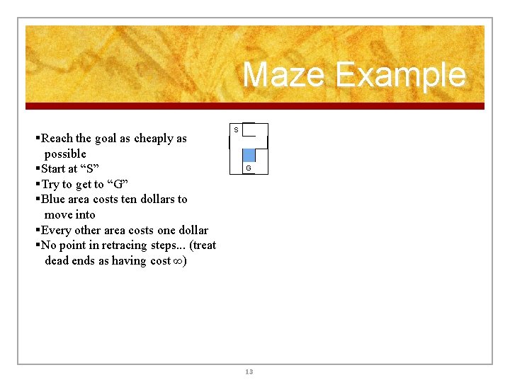
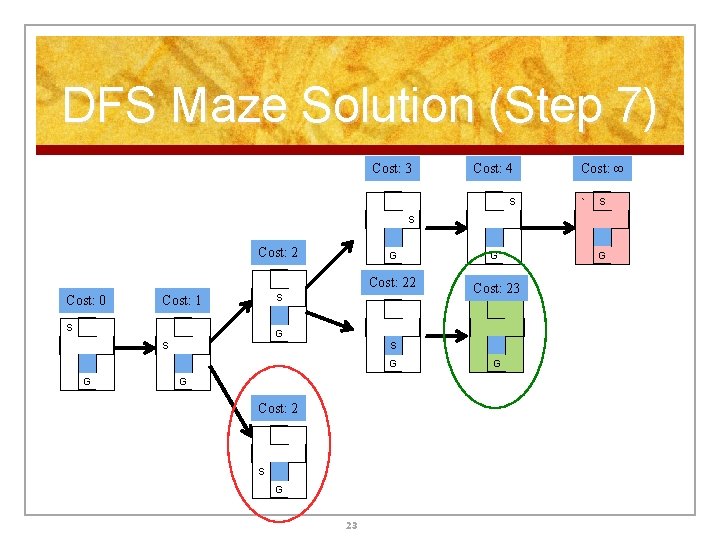
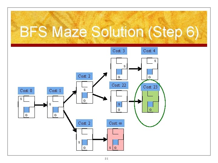
Maze Example §Reach the goal as cheaply as possible §Start at “S” §Try to get to “G” §Blue area costs ten dollars to move into §Every other area costs one dollar §No point in retracing steps. . . (treat dead ends as having cost ∞) S G 13

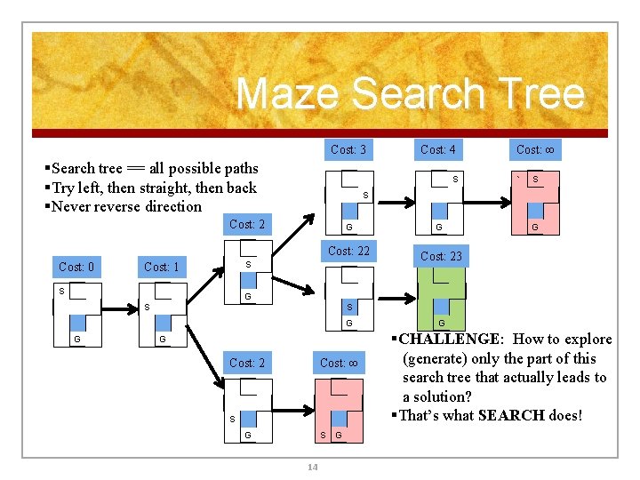
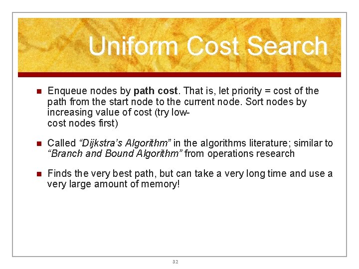
Maze Search Tree Cost: 3 §Search tree == all possible paths §Try left, then straight, then back §Never reverse direction S G Cost: 22 S Cost: 1 S Cost: ∞ ` S S Cost: 2 Cost: 0 Cost: 4 G G Cost: 23 G S S G G G Cost: 2 Cost: ∞ S G S 14 G G §CHALLENGE: How to explore (generate) only the part of this search tree that actually leads to a solution? §That’s what SEARCH does!

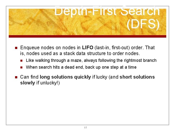
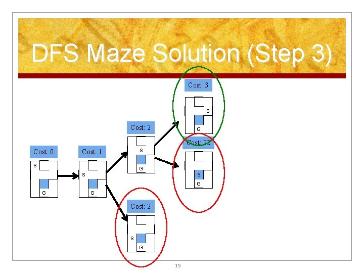
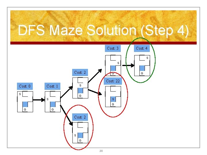
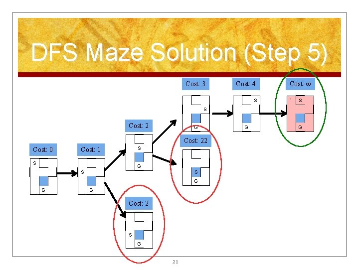
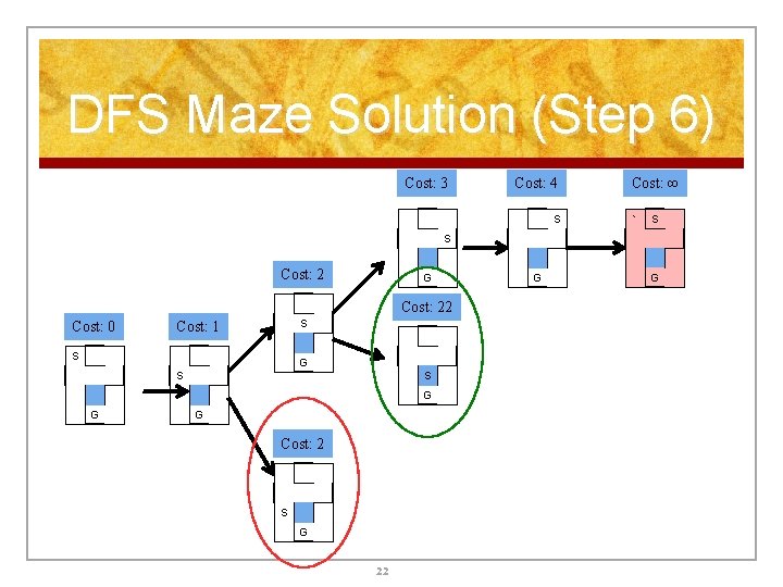
Depth-First Search (DFS) n n Enqueue nodes on nodes in LIFO (last-in, first-out) order. That is, nodes used as a stack data structure to order nodes. n Like walking through a maze, always following the rightmost branch n When search hits a dead end, back up one step at a time Can find long solutions quickly if lucky (and short solutions slowly if unlucky!) 15

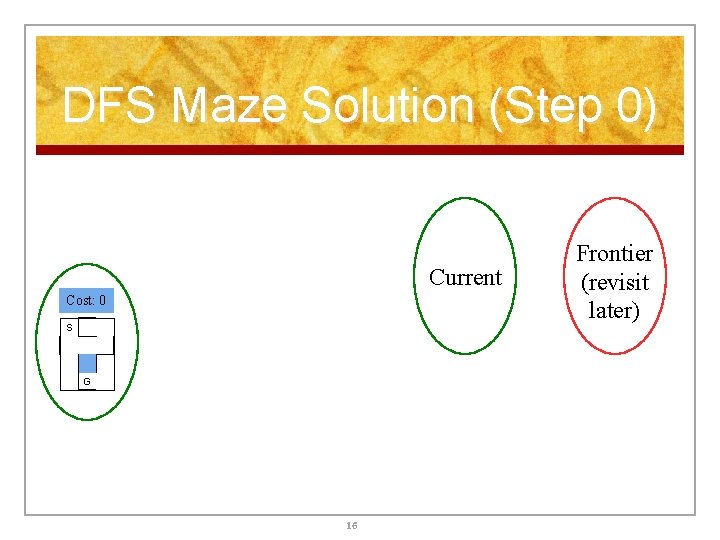
DFS Maze Solution (Step 0) Current Cost: 0 S G 16 Frontier (revisit later)

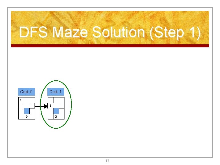
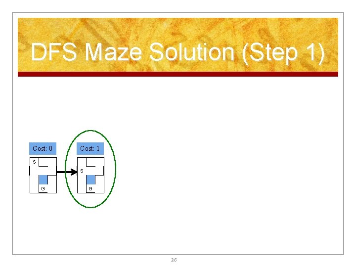
DFS Maze Solution (Step 1) Cost: 0 Cost: 1 S S G G 17

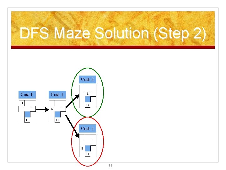
DFS Maze Solution (Step 2) Cost: 2 Cost: 0 S Cost: 1 S G G Cost: 2 S G 18

DFS Maze Solution (Step 3) Cost: 3 S Cost: 2 G Cost: 22 Cost: 0 S Cost: 1 S G S S G G G Cost: 2 S G 19

DFS Maze Solution (Step 4) Cost: 3 Cost: 4 S S Cost: 2 G Cost: 22 Cost: 0 S Cost: 1 S G S S G G G Cost: 2 S G 20 G

DFS Maze Solution (Step 5) Cost: 3 Cost: 4 S Cost: ∞ ` S S Cost: 2 G Cost: 22 Cost: 0 S Cost: 1 S G S S G G G Cost: 2 S G 21 G G

DFS Maze Solution (Step 6) Cost: 3 Cost: 4 S Cost: ∞ ` S S Cost: 2 G Cost: 22 Cost: 0 S Cost: 1 S G S S G G G Cost: 2 S G 22 G G

DFS Maze Solution (Step 7) Cost: 3 Cost: 4 S Cost: ∞ ` S S Cost: 2 G Cost: 22 Cost: 0 S Cost: 1 S G Cost: 23 G S S G G G Cost: 2 S G 23 G G

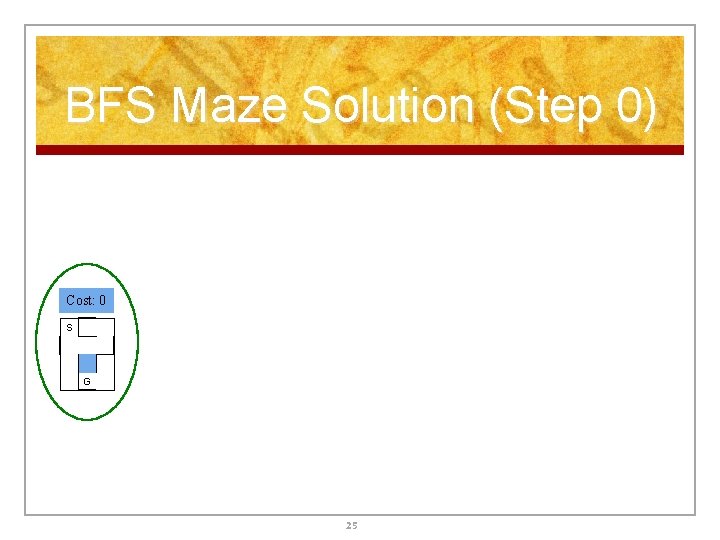
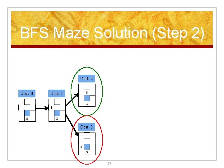
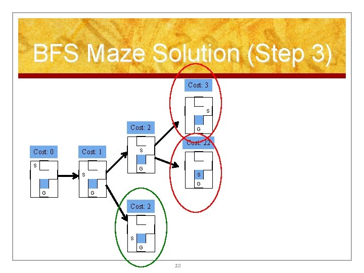
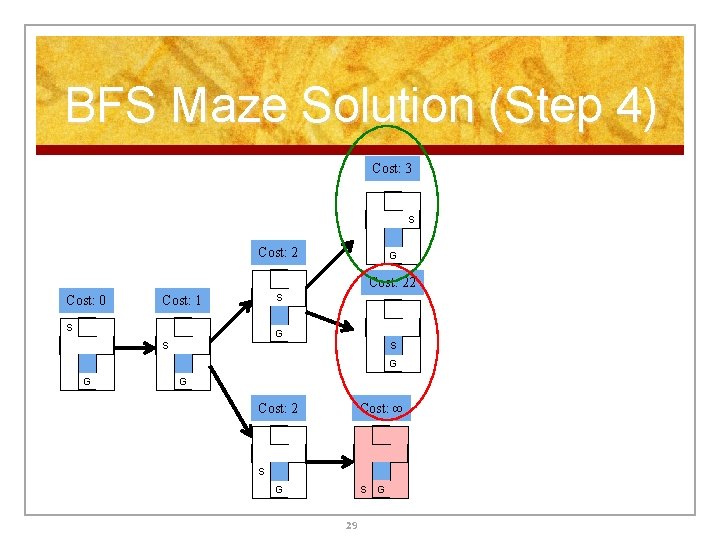
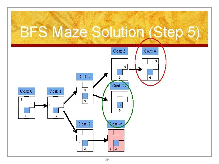
Breadth-First Search n Enqueue nodes on nodes in FIFO (first-in, firstout) order. n n n Like having a team of “gremlins” who can keep track of every branching point in a maze Only one gremlin can move at a time, and breadth-first search moves them each in turn, duplicating the gremlins if they reach a “fork in the road” – one for each fork! Finds the shortest path, but sometimes very slowly (and at the cost of generating lots of gremlins!) 24

BFS Maze Solution (Step 0) Cost: 0 S G 25

DFS Maze Solution (Step 1) Cost: 0 Cost: 1 S S G G 26

BFS Maze Solution (Step 2) Cost: 2 Cost: 0 S Cost: 1 S G G Cost: 2 S G 27

BFS Maze Solution (Step 3) Cost: 3 S Cost: 2 G Cost: 22 Cost: 0 S Cost: 1 S G S S G G G Cost: 2 S G 28

BFS Maze Solution (Step 4) Cost: 3 S Cost: 2 G Cost: 22 Cost: 0 S Cost: 1 S G S S G G G Cost: 2 Cost: ∞ S G S 29 G

BFS Maze Solution (Step 5) Cost: 3 Cost: 4 S S Cost: 2 G Cost: 22 Cost: 0 S Cost: 1 S G S S G G G Cost: 2 Cost: ∞ S G S 30 G G

BFS Maze Solution (Step 6) Cost: 3 Cost: 4 S S Cost: 2 G Cost: 22 Cost: 0 S Cost: 1 S G Cost: 23 G S S G G G Cost: 2 Cost: ∞ S G S 31 G G

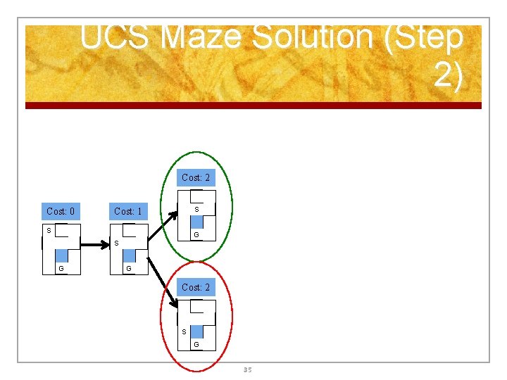
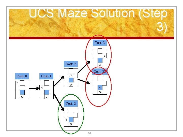
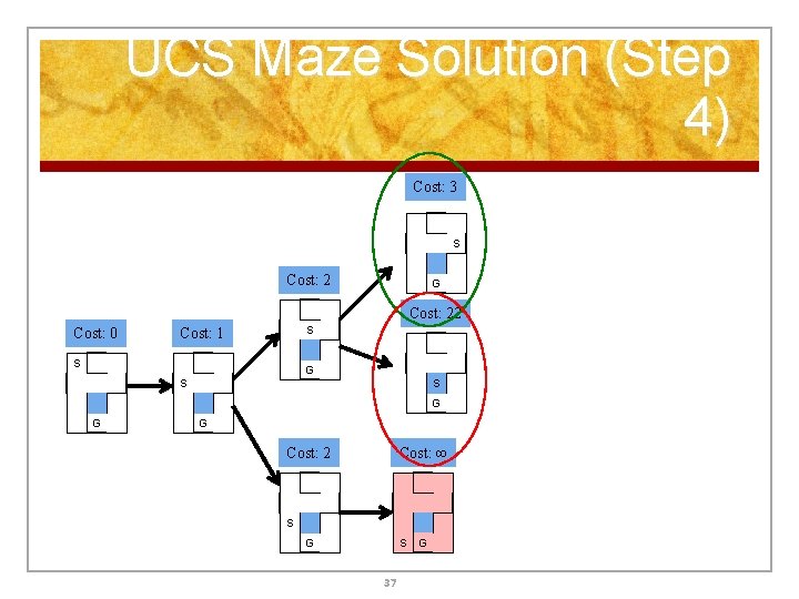
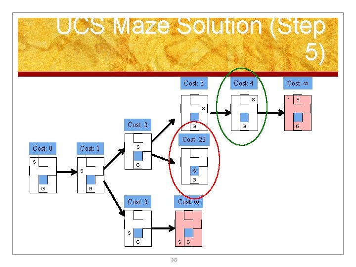
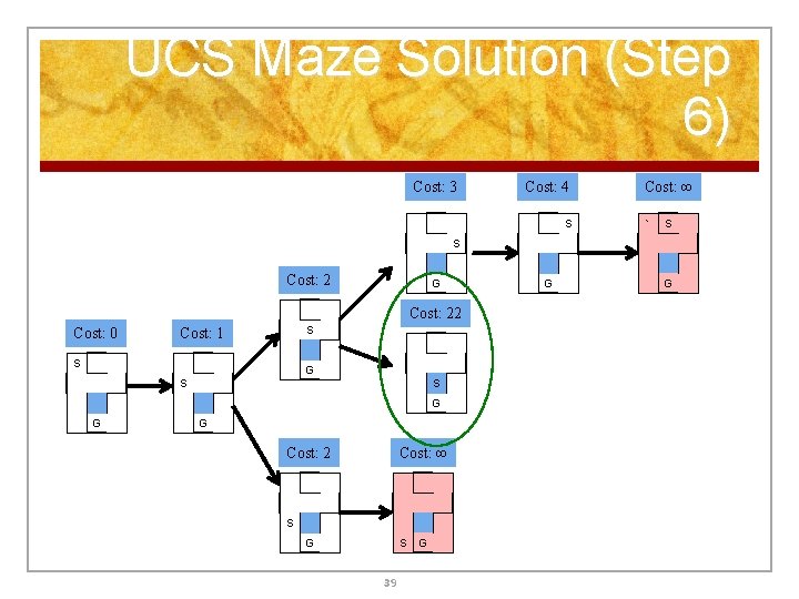
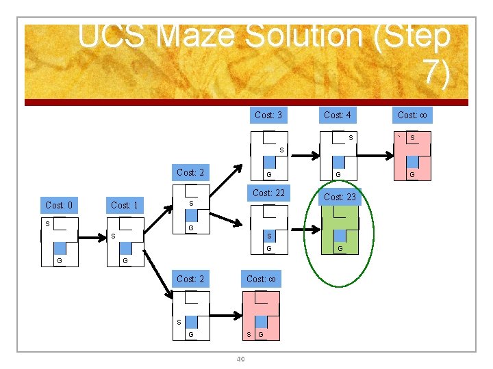
Uniform Cost Search n Enqueue nodes by path cost. That is, let priority = cost of the path from the start node to the current node. Sort nodes by increasing value of cost (try lowcost nodes first) n Called “Dijkstra’s Algorithm” in the algorithms literature; similar to “Branch and Bound Algorithm” from operations research n Finds the very best path, but can take a very long time and use a very large amount of memory! 32

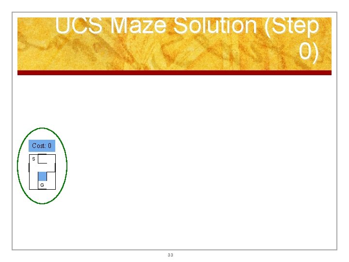
UCS Maze Solution (Step 0) Cost: 0 S G 33

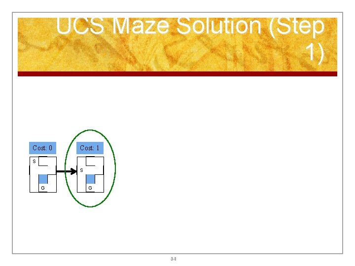
UCS Maze Solution (Step 1) Cost: 0 Cost: 1 S S G G 34

UCS Maze Solution (Step 2) Cost: 2 Cost: 0 S Cost: 1 S G G Cost: 2 S G 35

UCS Maze Solution (Step 3) Cost: 3 S Cost: 2 G Cost: 22 Cost: 0 S Cost: 1 S G S S G G G Cost: 2 S G 36

UCS Maze Solution (Step 4) Cost: 3 S Cost: 2 G Cost: 22 Cost: 0 S Cost: 1 S G S S G G G Cost: 2 Cost: ∞ S G S 37 G

UCS Maze Solution (Step 5) Cost: 3 Cost: 4 S Cost: ∞ ` S S Cost: 2 G Cost: 22 Cost: 0 S Cost: 1 S G S S G G G Cost: 2 Cost: ∞ S G S 38 G G G

UCS Maze Solution (Step 6) Cost: 3 Cost: 4 S Cost: ∞ ` S S Cost: 2 G Cost: 22 Cost: 0 S Cost: 1 S G S S G G G Cost: 2 Cost: ∞ S G S 39 G G G

UCS Maze Solution (Step 7) Cost: 3 Cost: 4 S Cost: ∞ ` S S Cost: 2 G Cost: 22 Cost: 0 S Cost: 1 S G Cost: 23 G S S G G G Cost: 2 Cost: ∞ S G S 40 G G G

Holy Grail Search If only we knew where we were headed… 41

Informed Search

What’s a Heuristic? From Word. Net (r) 1. 6 heuristic adj 1: (computer science) relating to or using a heuristic rule 2: of or relating to a general formulation that serves to guide investigation [ant: algorithmic] n : a commonsense rule (or set of rules) intended to increase the probability of solving some problem [syn: heuristic rule, heuristic program] 43

Informed Search: Use What You Know! n Add domain-specific information to select the best path along which to continue searching n Define a heuristic function that estimates how close a node n is to the goal node n Incorporate the heuristic function into search to choose the most promising branch along which to search: n Greedy search: Go in the most promising direction of any frontier node (ignoring how much it cost you to get to that frontier node) n A* search: Combine the work you’ve done so far to get to a frontier node, plus the heuristic estimate to the goal node, and pick the most promising in terms of total cost 44

Local Search

Local Search n Another approach to search involves starting with an initial guess at a solution and gradually improving it until it is a legal solution or the best that can be found. n Also known as “incremental improvement” search n Some examples: n Hill climbing n Genetic algorithms 46

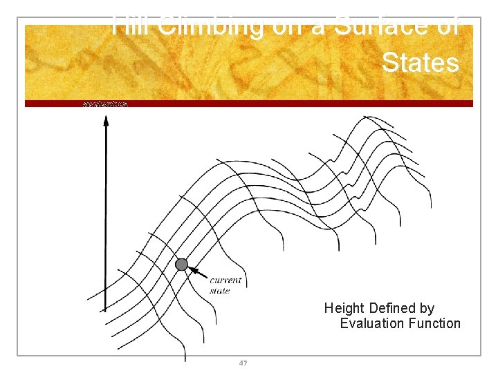
Hill Climbing on a Surface of States Height Defined by Evaluation Function 47

Drawbacks of Hill Climbing n n n Problems: n Local Maxima: peaks that aren’t the highest point in the space n Plateaus: the space has a broad flat region that gives the search algorithm no direction (random walk) n Ridges: flat like a plateau, but with dropoffs to the sides; steps to the North, East, South and West may go down, but a step to the NW may go up. Remedies: n Random restart n Problem reformulation Some problem spaces are great for hill climbing and others are terrible. 48

Genetic Algorithms n Start with k random states (the initial population) n New states are generated by “mutating” a single state or “reproducing” (combining) two parent states (selected according to their fitness) n Encoding used for the “genome” of an individual strongly affects the behavior of the search n Genetic algorithms / genetic programming are a large and active area of research 49

Game Playing

Why Study Games? n Clear criteria for success n Offer an opportunity to study problems involving {hostile, adversarial, competing} agents. n Historical reasons n Fun n Interesting, hard problems thatrequire minimal “initial structure” n Games often define very large search spaces n chess 35100 nodes in search tree, 1040 legal states 51

State of the Art n How good are computer game players? n n n Chess: § Deep Blue beat Gary Kasparov in 1997 § Garry Kasparav vs. Deep Junior (Feb 2003): tie! § Kasparov vs. X 3 D Fritz (November 2003): tie! http: //www. cnn. com/2003/TECH/fun. games/11/19/kasparov. chess. ap/ Checkers: Chinook (an AI program with a very large endgame database) is the world champion (checkers is “solved”!) Go: Computer players are competitive at a professional level Bridge: “Expert-level” computer players exist (but no world champions yet!) Poker: Computer team beat a human team, using statistical modeling and adaptation: http: //www. cs. ualberta. ca/~games/poker/man-machine/ Good places to learn more: n n http: //www. cs. ualberta. ca/~games/ http: //www. cs. unimass. nl/icga 52

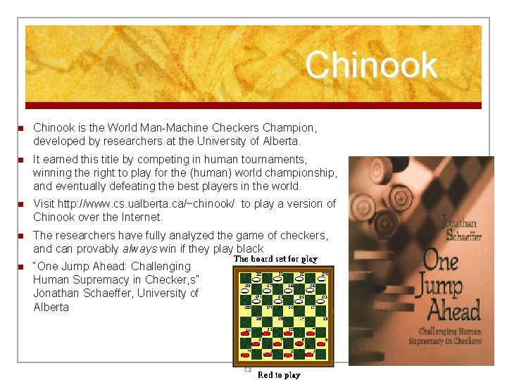
Chinook n Chinook is the World Man-Machine Checkers Champion, developed by researchers at the University of Alberta. n It earned this title by competing in human tournaments, winning the right to play for the (human) world championship, and eventually defeating the best players in the world. n Visit http: //www. cs. ualberta. ca/~chinook/ to play a version of Chinook over the Internet. n The researchers have fully analyzed the game of checkers, and can provably always win if they play black n “One Jump Ahead: Challenging Human Supremacy in Checker, s” Jonathan Schaeffer, University of Alberta 53

Typical Game Setting n 2 -person game n Players alternate moves n Zero-sum: one player’s loss is the other’s gain n Perfect information: both players have access to complete information about the state of the game. No information is hidden from either player. n No chance (e. g. , using dice) involved n Examples: Tic-Tac-Toe, Checkers, Chess, Go, Nim, Othello n Not: Bridge, Solitaire, Backgammon, . . . 54

Let’s Play Nim! n Seven tokens (coins, sticks, whatever) n Each player must take either 1 or 2 tokens n Whoever takes the last token loses n You can go first… 55

How to Play a Game n n A way to play such a game is to: n Consider all the legal moves you can make n Compute the new position resulting from each move n Evaluate each resulting position and determine which is best n Make that move n Wait for your opponent to move and repeat Key problems are: n Representing the “board” n Generating all legal next boards n Evaluating a position 56

Evaluation Function n Evaluation function or static evaluator is used to evaluate the “goodness” of a game position. n n Contrast with heuristic search where the evaluation function was a non-negative estimate of the cost from the start node to a goal and passing through the given node The zero-sum assumption allows us to use a single evaluation function to describe the goodness of a board with respect to both players. n f(n) >> 0: position n good for me and bad for you n f(n) << 0: position n bad for me and good for you n f(n) near 0: position n is a neutral position n f(n) = +infinity: win for me n f(n) = -infinity: win for you 57

Evaluation Function Examples n Example of an evaluation function for Tic-Tac-Toe: f(n) = [# of 3 -lengths open for me] - [# of 3 -lengths open for you] where a 3 -length is a complete row, column, or diagonal n Alan Turing’s function for chess n n f(n) = w(n)/b(n) where w(n) = sum of the point value of white’s pieces and b(n) = sum of black’s Most evaluation functions are specified as a weighted sum of position features: f(n) = w 1*feat 1(n) + w 2*feat 2(n) +. . . + wn*featk(n) n n Example features for chess are piece count, piece placement, squares controlled, etc. Deep Blue had over 8000 features in its evaluation function 58

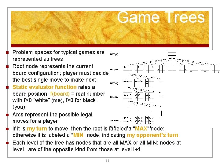
Game Trees n n n Problem spaces for typical games are represented as trees Root node represents the current board configuration; player must decide the best single move to make next Static evaluator function rates a board position. f(board) = real number with f>0 “white” (me), f<0 for black (you) Arcs represent the possible legal moves for a player If it is my turn to move, then the root is labeled a "MAX" node; otherwise it is labeled a "MIN" node, indicating my opponent's turn. Each level of the tree has nodes that are all MAX or all MIN; nodes at level i are of the opposite kind from those at level i+1 59

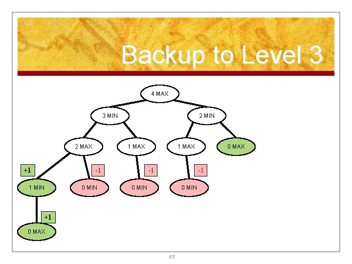
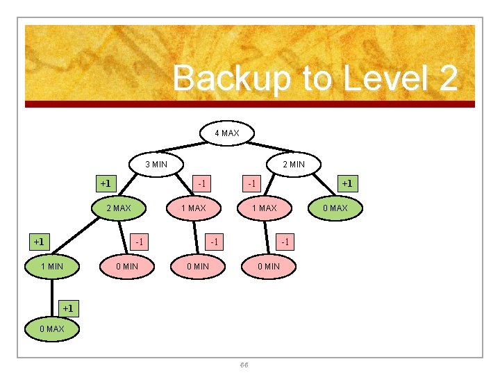
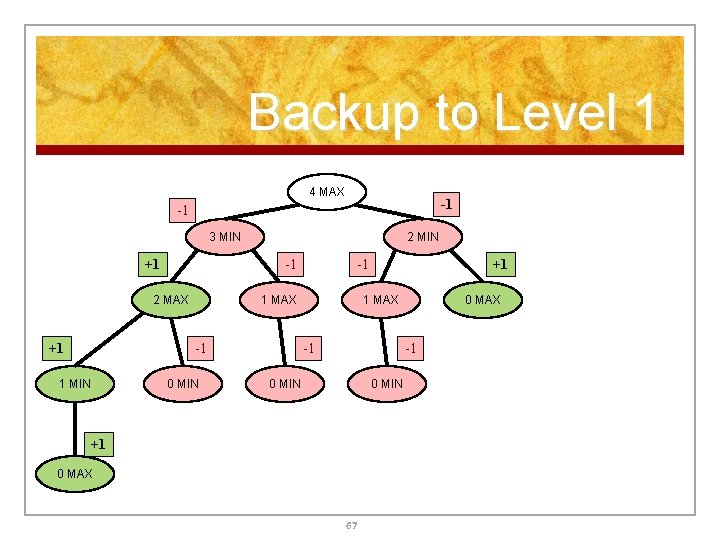
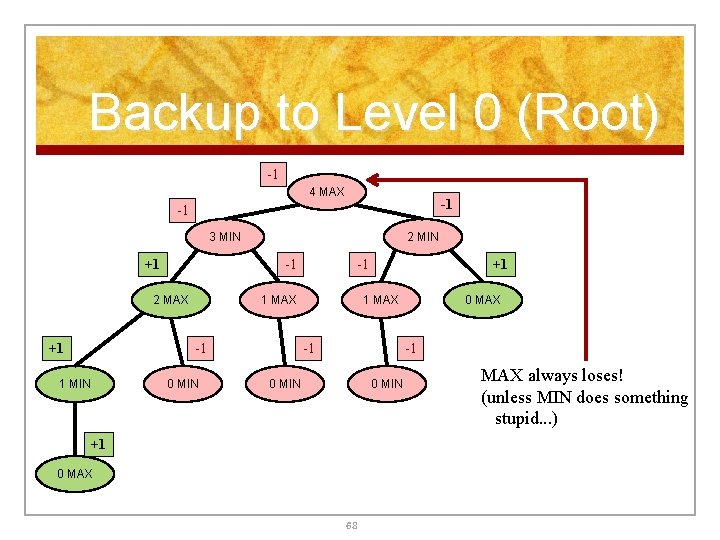
Minimax Procedure n Create start node as a MAX node with current board configuration n Expand nodes down to some depth (a. k. a. ply) of lookahead in the game n Apply the evaluation function at each of the leaf nodes n “Back up” values for each of the non-leaf nodes until a value is computed for the root node n n n At MIN nodes, the backed-up value is the minimum of the values associated with its children. (Best move for the MIN player) At MAX nodes, the backed-up value is the maximum of the values associated with its children. (Best move for the MAX player) Pick the operator associated with the child node whose backed 60 at the root up value determined the value

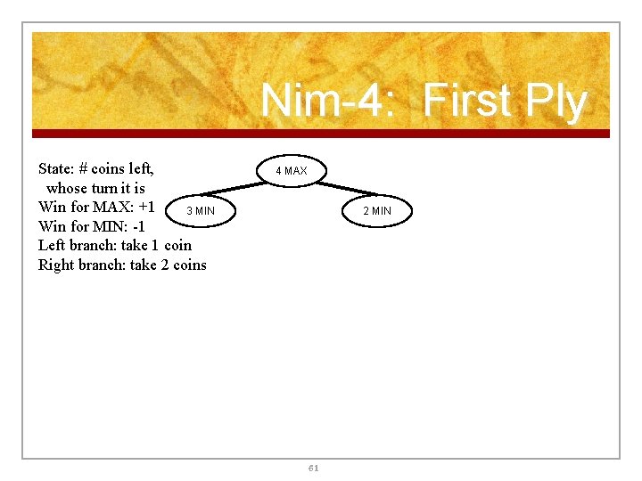
Nim-4: First Ply State: # coins left, whose turn it is Win for MAX: +1 3 MIN Win for MIN: -1 Left branch: take 1 coin Right branch: take 2 coins 4 MAX 2 MIN 61

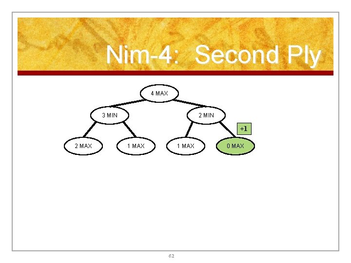
Nim-4: Second Ply 4 MAX 3 MIN 2 MIN +1 2 MAX 1 MAX 62 0 MAX

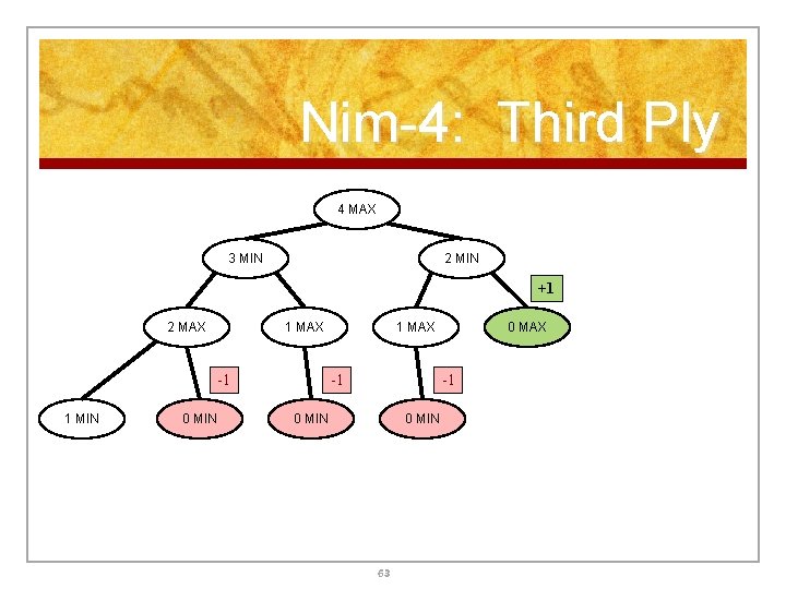
Nim-4: Third Ply 4 MAX 3 MIN 2 MIN +1 2 MAX 1 MAX -1 1 MIN 0 MIN 1 MAX -1 0 MIN 63

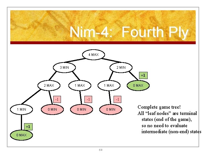
Nim-4: Fourth Ply 4 MAX 3 MIN 2 MIN +1 2 MAX 1 MAX -1 1 MIN 0 MIN 1 MAX -1 0 MIN +1 0 MAX 64 Complete game tree! All “leaf nodes” are terminal states (end of the game), so no need to evaluate intermediate (non-end) states

Backup to Level 3 4 MAX 3 MIN 2 MAX +1 2 MIN 1 MAX -1 1 MIN 0 MIN 1 MAX -1 0 MIN +1 0 MAX 65

Backup to Level 2 4 MAX 3 MIN +1 -1 2 MAX +1 2 MIN 1 MAX -1 1 MIN -1 0 MIN +1 1 MAX -1 0 MIN +1 0 MAX 66

Backup to Level 1 4 MAX -1 -1 3 MIN +1 -1 2 MAX +1 2 MIN 1 MAX -1 1 MIN -1 0 MIN +1 1 MAX -1 0 MIN +1 0 MAX 67

Backup to Level 0 (Root) -1 4 MAX -1 -1 3 MIN +1 -1 2 MAX +1 2 MIN 1 MAX -1 1 MIN -1 0 MIN +1 1 MAX -1 0 MIN +1 0 MAX 68 MAX always loses! (unless MIN does something stupid. . . )